DCF Myth 3.2: If you don't look, its not there!

Setting the Stage

The tools that we use in finance were developed in simpler times, when data was often difficult (or expensive) to access and sophisticated statistical tools required machine power that was beyond the reach of most in the finance community. It should come as no surprise then that in discounted cash flow valuation, we have historically used point estimates ( single numbers that reflect best judgments at the time of the valuation) for variables that have probability distributions attached to them. To illustrate, in my valuation of Apple in February 2016, I used a revenue growth rate of 2.2% and a target operating margin of 25%, to arrive at my estimate of value per share of $129.80.

It goes without saying (but I will say it anyway) that I will be wrong on both these numbers, at least in hindsight, but there is a more creative way of looking at this estimation concern. Rather than enter a single number for each variable, what if I were able to enter a probability distribution? Thus, my estimate for revenue growth would still have an expected value of 2.2% (since that was my best estimate) but would also include a probability distribution that reflected my uncertainty about that value. That distribution would capture not only the magnitude of my uncertainty (in a variance or a standard deviation) but also which direction I expect to be wrong more often (whether the growth is more likely to be lower than my expected value or higher).  Similarly, the expected value for the operating margin can stay at 25% but I can build in a range that reflects my uncertainty about this number.

Once you input the variables as distributions, you have laid the foundations for a probabilistic valuation or more specifically, for a simulation, where in each run, you pick one outcome out of each distribution (which can be higher or lower than your expected values) and estimate a value for the company based on the drawn outcomes. Once you have run enough simulations, your output will be a distribution of values across simulations. If the distributions of your variables are built around expected values that match up to the numbers that you used in your point estimate valuation, the expected value across the simulations will be close to your point estimate value. That may seem to make the simulation process pointless, but there are side benefits that you get from simulations that enrich your decision process. In addition to the expected value, you will get a measure of how much variability there is in this value (and thus the risk you face), the likelihood that you could be wrong in your judgment of whether the stock is under and over valued and the potential payoffs to be right and wrong. 

Statistical Distributions: A Short Preview

It is a sad truth that most of us who go through statistics classes quickly consign them to the “I am never going to use this stuff” heap and move on, but there is no discipline that is more important in today’s world of big data and decision making under uncertainty. If you are one of those fortunate souls who not only remembers your statistics class fondly but also the probability distributions that you encountered during the class, you can skip this section. If, like me, the only memory you have of your statistics class is of a bell curve and a normal distribution, you need to expand your statistical reach beyond a normal distribution, because much of what happens in the real world (which is what you use probability distributions to capture) is not normally distributed. At the risk of over simplifying the choices, here are some basic classifications of uncertainties/ risks::

1. Discrete versus Continuous Distributions: Assume that you are valuing an oil company in Venezuela and that you are concerned that the firm may be nationalized, a risk that either occurs or does not, i.e., a discrete risk. In contrast, the oil company's earnings will move with oil prices but take on a continuum of values, making it a continuous risk. With currency risk, the risk of devaluation in a fixed exchange rate currency is discrete risk but the risk in a floating rate currency is continuous.
2. Symmetric versus Asymmetric Distributions (Symmetric, Positive skewed, Negative skewed): While we don't tend to think of upside risk, risk can deliver outcomes that are better than expected or worse than expected. If the magnitude and likelihood of positive outcomes and negative outcomes is similar, you have a symmetric distribution. Thus, if the expected operating margin for Apple is 25% and can vary with equal probability from 20% to 30%, it is symmetrically distributed. In contrast, if the expected revenue growth for Apple is 2%, the worse possible outcome is that it could drop to -5%, but there remains a chance (albeit a small one) that revenue growth could jump back to 25% (if Apple introduces a disruptive new product in a big market), you have an a positively skewed distribution. In contrast, if the expected tax rate for a company is 35%, with the maximum value equal to the statutory tax rate of 40% (in the US) but with values as low as 0%, 5% or 10% possible (though not likely), you are looking at a negatively skewed distribution.
3. Extreme outcome likelihood (Thin versus Fat Tails): There is one final contrast that can be drawn between different risks. With some variables, the values will be clustered around the expected value and extreme outcomes, while possible, don't occur very often; these are thin tail distributions. In contrast, there are other variables, where the expected value is just the center of the distribution and actual outcome that are different from the expected value occur frequently, resulting in fat tail distributions.

I know that this is a very cursory breakdown, but if you are interested, I do have a short paper on the basics of statistical distributions (link below), written specifically with simulations in mind. 

Simulation Tools

I was taught simulation in my statistics class, the old fashioned way. My professor came in with three glass jars filled with little pieces of paper, with numbers written on them, representing the different possible outcomes on each variable in the problem (and I don't even remember what the problem was). He then proceeded to draw one piece of paper (one outcome) out of each jar and worked out the solution, with those numbers and wrote it on the board. I remember him meticulously returning those pieces of paper back into the jar (sampling with replacement) and at the end of the class, he proceeded to compute the distribution of his solutions.

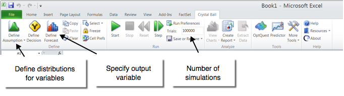
While the glass jar simulation is still feasible for simulating simple processes with one or two variables that take on only a few outcomes, it is not a comprehensive way of simulating more complex processes or continues distributions. In fact, the biggest impediment to using simulation until recently would have been the cost of running one, requiring the use of a mainframe computer. Those days are now behind us, with the evolution of technology both in the form of hardware (more powerful personal computers) and software. Much as it is subject to abuse, Microsoft Excel has become the lingua franca of valuation, allowing us to work with numbers with ease. There are some who are conversant enough with Excel's bells and whistles to build simulation capabilities into their spreadsheets, but I am afraid that I am not one of those. Coming to my aid, though, are offerings that are add-ons to Excel that allow for the conversion of any Excel spreadsheet almost magically into a simulation.

I normally don't make plugs for products and services, even if I like them, on my posts, because I am sure that you get inundated with commercial offerings that show up insidiously in Facebook and blog posts. I am going to make an exception and praise Crystal Ball, the Excel add-on that I use for simulations. It is an Oracle product and you can get a trial version by going here. (Just to be clear, I pay for my version of Crystal Ball and have no official connections to Oracle.) I like it simply because it is unobtrusive, adding a menu item to my Excel toolbar, and has an extremely easy learning curve.

My only critique of it, as a Mac user, is that it is offered only as a PC version and I have to run my Mac in MS Windows, a process that I find painful. I have also heard good things about @Risk, another excel add-on, but have not used it.

Simulation in Valuation

There are two aspects of the valuation process that make it particularly well suited to Monte Carlo simulations. The first is that uncertainty is the name of the game in valuation, as I noted in my first post in the series. The second is that valuation inputs are often estimated from data, and that data can be plentiful at least on some variables, making it easier to estimate the probability distributions that lie at the heart of simulations. The sequence is described in the picture below:

Step 1: Start with a base case valuation
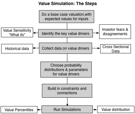
The first place to start a simulation is with a base case valuation. In a base case valuation, you do a valuation with your best estimates for the inputs into value from revenue growth to margins to risk measures. Much as you will be tempted to use conservative estimates, you should avoid the temptation and make your judgments on expected values. In the case of Apple, the numbers that I use in my base case valuation are very close to those that I used just a couple of months ago, when I valued the company after its previous earnings report and are captured in the picture below:

Download spreadsheet

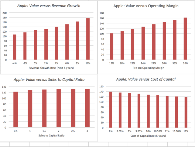
In my base case, at least, it looks like Apple is significantly under valued, priced at $93/share, with my value coming in at $126.47, just a little bit lower my valuation a few months ago. I did lower my revenue growth rate to 1.50%, reflecting the bad news about revenues in the most recent 10q.

Step 2: Identify your driver variables

As you can see the sales to capital ratio has little effect on value per share, largely because the base case growth rate that I use for Apple is so low. Revenue growth and operating margin both affect value significantly and cost of capital to a much lesser degree. Note that the value per share is higher than the current price though every single what-if analysis, but that reflects the fact that only variable at a time in being changed in this analysis. It is entirely possible that if both revenue growth and operating margins drop at the same time, the value per share will be lower than $93 (the stock price at the time of this analysis) and one of the advantages of a Monte Carlo simulation is that you can build in interconnections between variables. Looking at the variables through the lens that investors have been using to drive the stock price down, it seems like the front runner for value driver has to be revenue growth, as Apple reported its first year on year negative revenue growth in the last quarter and concerns grow about whether the iPhone franchise is peaking. Following next on the value driver list is the operating margin, as the competition in the smart phone business heats up.

Step 3: The Data Assessment

1. Past data: If the value driver is a macroeconomic variable, say interest rates or oil prices, you can draw on historical data going back in time. My favored site for all things macroeconomic is FRED, the Federal Reserve data site in St. Louis, a site that combines great data with an easy interface and is free. I have included data on interest rate, inflation, GDP growth and the weighted dollar for those of you interested in US data in the attached link. For data on other countries, currencies and markets, you can try the World Bank data base, not as friendly as FRED, but rich in its own way.
2. Company history: For companies that have been in existence for a long time, you can mine the historical data to get a measure of how key company-specific variables (revenues, operating margin, tax rate) vary over time. 
3. Sector data: You can also look at cross sectional differences in key variables across companies in a sector. Thus, to estimate the operating margin for Amazon, you could look at the distribution of margins across retail companies.: If the value driver is a macroeconomic variable, say interest rates or oil prices, you can draw on historical data going back in time. My favored site for all things macroeconomic is FRED, the Federal Reserve data site in St. Louis, a site that combines great data with an easy interface and is free. I have included data on interest rate, inflation, GDP growth and the weighted dollar for those of you interested in US data in the attached link. For data on other countries, currencies and markets, you can try the World Bank data base, not as friendly as FRED, but rich in its own way.

Step 4: Distributional Assumptions
There is no magic formula for converting the data that you have collected into probability distributions, and as with much else in valuation, you have to make your best judgments on three dimensions.

1. Distribution Type: In the section above, I broadly categorized the uncertainties you face into discrete vs continuous, symmetric vs skewed and fat tail vs thin tail. At the risk of being tarred and feathered for bending statistical rules, I have summarized the distribution choices based on upon these categorizations. The picture is not comprehensive but it can provide a road map though the choices:
   
   
2. Distribution Parameters: Once you have picked a distribution, you will have to input the parameters of the distribution. Thus, if you had the good luck to have a variable be normally distributed, you will only be asked for an expected value and a standard deviation. As you go to more complicated distributions, one way to assess your parameter choices to look at the full distribution, based upon your parameter choices, and pass it through the common sense test.

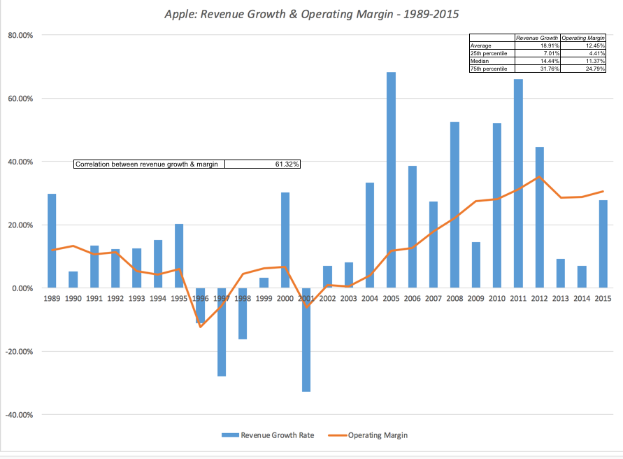
In the case of Apple, I will use the historical data from the company, the cross sectional distribution of revenue growth across older technology companies as well as a healthy dose of subjective reasoning to pick a lognormal distribution, with parameters picked to yield values ranging from -4% on the downside to +10% on the upside. On the target operating margin, I will build my distribution around the 25% that I assumed in my base case and assume more symmetry in the outcomes; I will use a triangular distribution to prevent even the outside chance of infinite margins in either direction.

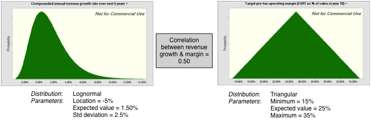
Note the correlation between the two, which I will talk about in the next section.

Step 5: Build in constraints and correlations
There are two additional benefits that come with simulations. The first is that you can build in constraints that will affect the company's operations, and its value, that are either internally or externally imposed. For an example of an external constraint, consider a company with a large debt load. That does not apply to Apple but it would to Valeant. If the company's value drops below the debt due, you could set the equity value to zero, on the assumption that the company will be in default. As another example, assume that you are valuing a bank and that you model regulatory capital requirements as part of your valuation. If the regulatory capital drops below the minimum required, you can require the company to issue more shares (thus reducing the value of your equity).  The second advantage of a simulation is that you can build in correlations across variables, making it more real life. Thus, if  you believe that bad outcomes on margins (lower margins than expected) are more likely to go with bad outcomes on revenue growth (revenue growth lower than anticipated), you can build in a positive correlation between the variables. With Apple, I see few binding constraints that will affect the valuation. The company has little chance of default and is not covered by regulatory constraints on capital. I do see revenues and operating margins moving together and I build in this expectation by assuming a correlation of 0.50 (lower than the historical correlation of 0.61 between revenues and operating margin from 1989 to 2015 at Apple).

Step 6: Run the simulations

Using my base case valuation of Apple (which yielded the value per share of $126.47) as my starting point and inputting the distributional assumptions for revenue growth and operating margin, as well as the correlation between the two, I used Crystal Ball to run the simulations (leaving the number at the default of 100,000) and generated the following distribution for value:

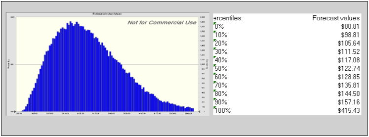
The percentiles of value and other key statistics are listed on the side. Could Apple be worth less than $93/share. Yes, but the probability is less than 10%, at least based on my assumptions. Having bought and sold Apple three times in the last six years (selling my shares last summer), this is undoubtedly getting old, but I am an Apple shareholder again. I am not a diehard believer in the margin of safety, but if I were, I could use this value distribution to create a more flexible version of it, increasing it for companies with volatile value distributions and reducing it for firms with more stable ones.

The most serious concern that I have, as an investor, is that I am valuing cash , which at $232 billion is almost a third of my estimated value for Apple, as a neutral asset (with an expected tax liability of $28 billion). Some of you, who have visions of Apple disrupting new businesses with the iCar or the iPlane may feel that this is too pessimistic and that there should be a premium attached for these future disruptions. My concern is the opposite, i.e., that Apple will try to do too much with its cash, not too little. In my post on aging technology companies, I argued that, like aging movie stars in search of youth, some older tech companies throw money at bad growth possibilities. With the amount of money that Apple has to throw around, that could be deadly to its stockholders and I have to hope and pray that the company remains restrained, as it has been for much of the last decade.

Conclusion