Demand
A desire or willingness to buy certain goods or services backed by the ability to pay for them at a specific price.


What Is Demand?
In economics, Demand (D) is a desire or willingness to buy certain goods or services backed by the ability to pay for them at a specific price. It is a relationship between the market price and the quantity demanded (QD).
According to Cambridge Dictionary, the word demand has several meanings. It can have a form of a noun or a verb.
One of its meanings as a verb is, for example, to ask for something forcefully. On the other hand, its noun meanings are related to a strong request or need for something, for example, goods or services. The latter definition is the closest to the one used in economics.
Economists use the demand abbreviation D; for market demand, it is capital D, and for individual need, it is "d."
Because customers are willing to purchase different amounts of goods and services at different prices, economists developed further specific terms discussed below to express the general concepts of D.
Whether the relationship between the price and quantity is positive or negative (or inverse) is determined by the law of demand, also called the law of downward-sloping demand.
The Law of D states that the QD will decrease with the increasing price of a good or service. This is valid for almost all goods and services, and countless empirical studies confirm it.
Further terms that define the concept of D are represented by the demand:
- function
- schedule
- curve
A demand schedule is a statistical representation of D. It is a table that shows the demanded quantity of goods or services for various market prices (if other circumstances are unchanged). Below is an illustration of how the D schedule could look:
| Price in $ | 4 | 5 | 6 | 7 | 8 |
|---|---|---|---|---|---|
| Quantity demanded (QD) | 40 | 35 | 30 | 25 | 20 |
On a graph with the axis x representing quantity and the axis y representing price, D is projected on a demand curve. The D curve is a graphical representation of the relationship between the market price and the QD.
Economists draw the D curve as a smooth continuous curve, either as
- straight (linear line) or
- curved (non-linear) line.
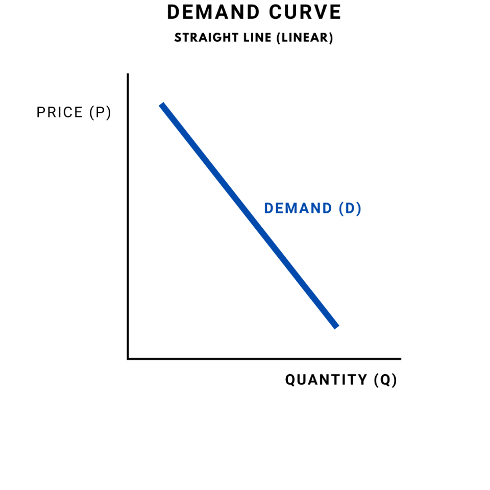
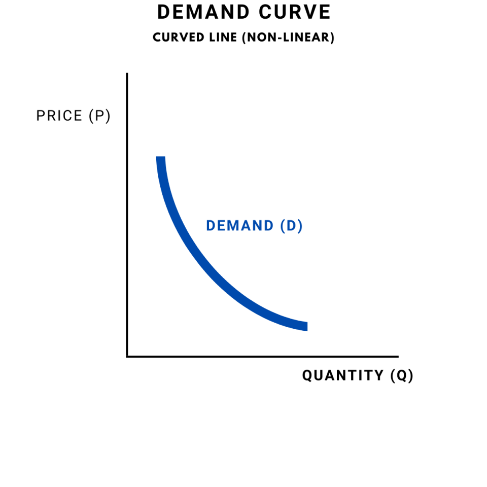
Due to the law of demand, the D curve slopes downwards. The mathematical representation of D and its curve is called the demand function;
Q = a + bP
or
q = f(x)
Economists often use a representation in the form of an inverse demand function:
P = a + Qb
or
p = f(x)
The main difference between the D function and the inverse D function is the variables placed on the horizontal axis x and the vertical axis y. For example, the D function puts the quantity (Q) on the vertical axis y, and the price (P) on the horizontal axis x.
However, in most cases, economists put the price (P) on the vertical axis y and quantity (Q) on the horizontal axis x. Therefore, using the inverse D function: P= a + Qb, or mathematically p=f(x), is more practical and accurate.
According to the textbook Economics, the market demand curve (D) is a sum of individual demands (d). It is therefore found by adding all the quantities demanded by all individuals for the given price
constructing a demanding schedule
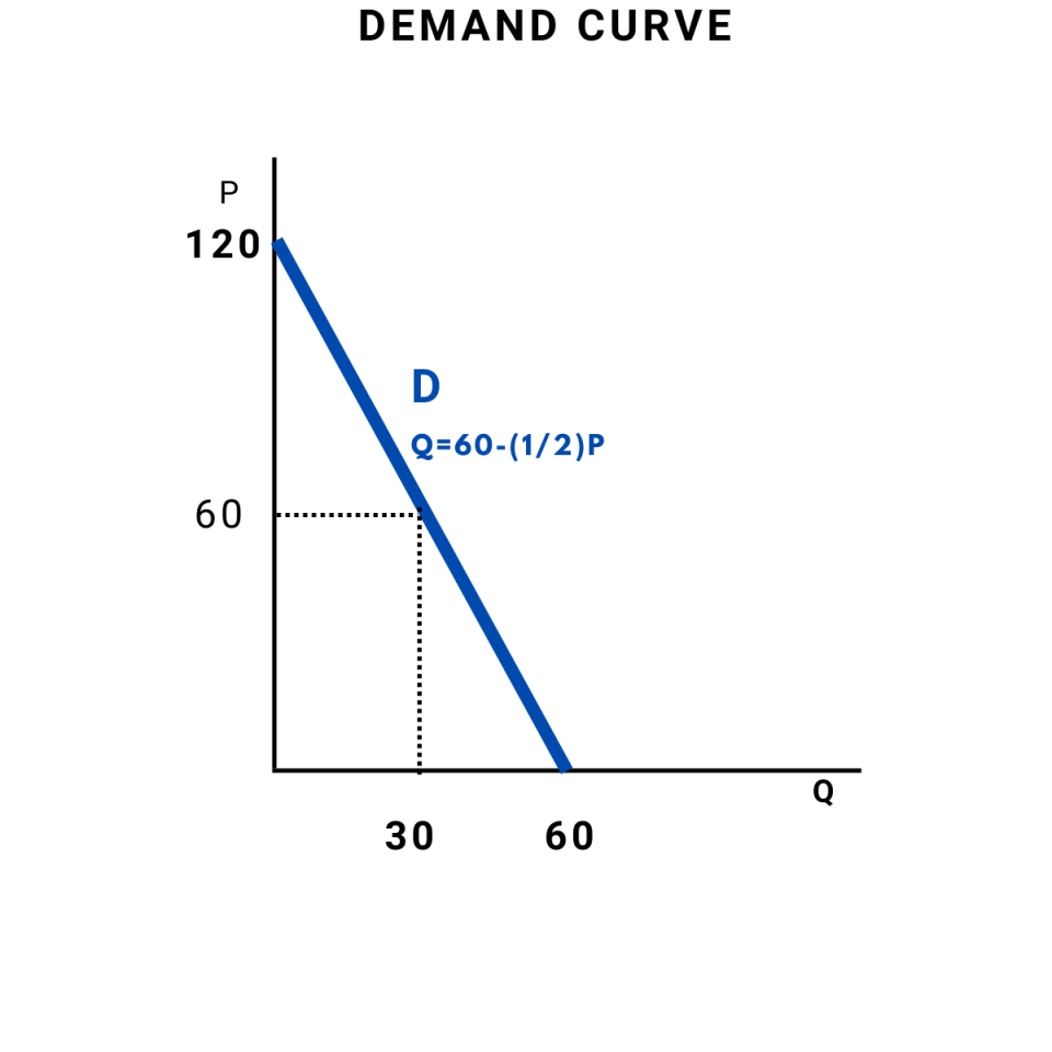
The D function determines its curve and the schedule. Let us consider an example to demonstrate how to build the D curve and create a D schedule from the D function. Our D function is Q = 60 − (½)P. Therefore, the inverse D function is P = 120 − 2Q.
To draw a curve for this particular function, we need to determine the x and y-intercepts. The x-intercept is when Q=0 and it is calculated as follows:
0 = 60-(½)P
(½)P=60
P=120
The y-intercept is when P=0, and it is calculated as follows:
0=120-2Q
2Q=120
Q=60
We can draw the curve as a straight line based on these findings, as our function is linear. Also, our turn will start at the point P=120 and end at the point Q=60. The angle is illustrated below:
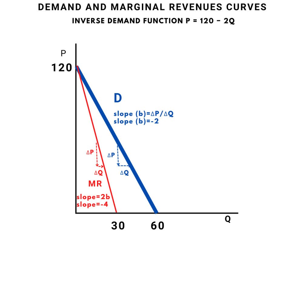
To determine the slope of the D curve, we will consider the general inverse D function P=a+bQ, where the b coefficient represents the slope. In our example, where our inverse function is P = 120 − 2Q, the hill will be -2.
The negative slope occurs when there is an inverse relationship between the variables. The price and quantity move in opposite directions, which aligns with the D law.
In economic analysis, a widely used law is applied to the linear D function related to its slope. The marginal revenue (MR) curve's slope is twice as steep as the D curve. Therefore, we can also draw a marginal revenue curve from our case's information.
The general calculus proof of the rule, computing the marginal revenues (MR) from the total revenues (TR) using derivatives rules:
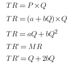
The calculus proof using our example inverse D function:
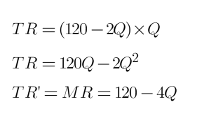
The evidence shows that the marginal revenue curve would start at the same point as the D curve. However, it would end at the point Q=30, as its slope is twice as steep as the D curve's slope; -4.
The derivatives rules used in this calculus were as follows:
- Power rule
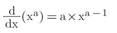
- The derivative of a differentiation variable is 1. Furthermore, we can fill in our schedule by calculating the QD related to the individual price from the D function. The D schedule for our example is as follows:
Example Price 0 10 40 60 100 120 Quantity demanded 60 55 40 30 10 0
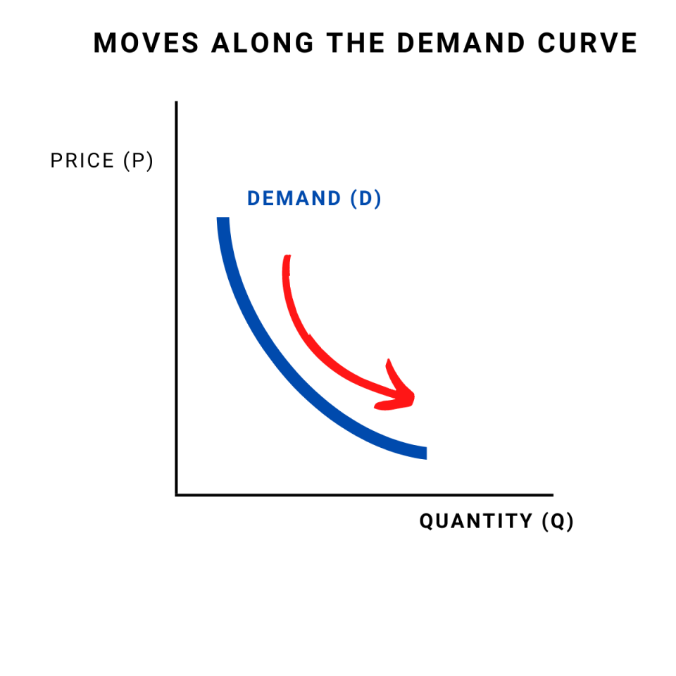
Movement along the demand Curves and shifts in demand
When talking about the changes in D, we need to identify whether the changes in demanded quantity are also accompanied by a difference in the price or not. Based on this observation, we distinguish two differences:
- Movement along the D curve (change in demanded price and quantity).
- Shifts of the D curve (changes in demand).
A movement along a D curve that results from a price change is called a change in demanded quantity and price. We are not talking here about the change in demand but rather about the increase or decrease in the required amount.
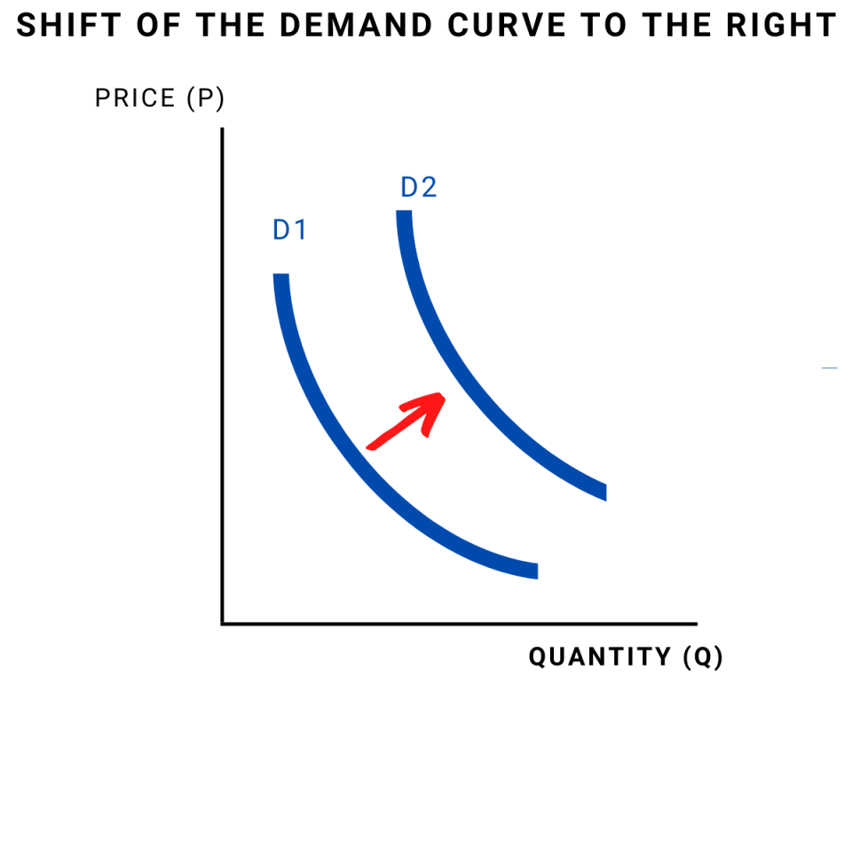
Shifts of the D curve to the left or the right represent a change in demand. When there is a decrease in need, the D curve moves to the left.
Similarly, when there is an increase in demand, the D curve shifts to the right. Changes in order are characterized by changes in demanded quantity when the price is unchanged.
As stated in the Introduction to Economic Analysis, an increase in D is represented by a movement of the entire curve to the northeast (up and to the right), which represents an increase in the marginal value v (move up) for any given unit or an increase in the number of units demanded any given price (move to the right).
Factors Of Shifts in Demand
A demand shifter is a factor that can change the quantity of a good or service demanded at each price.
Different factors will impact the D for other goods and services. However, some universal influencing factors are also called D shifters. The most common D shifters are:
- consumer preferences,
- the prices of related goods and services,
- income,
- demographic characteristics, and
- buyer expectations.
Consumer Preferences
The consumer has great power over the influence of the D. If consumers' preferences change and they do not prefer the product or service; they will decrease D and shift the D curve to the left.
If the consumers start to prefer a particular product or service, the D will increase, and the D curve will shift to the right.
The Prices Of Related Goods And Services
In case those two are related, the prices of other goods and services could affect the D for specific goods or services. There are two ways goods and services could be told in two ways:
- As complements or
- As substitutes.
If two goods are complements, the increased D for one good will increase the D for the other.
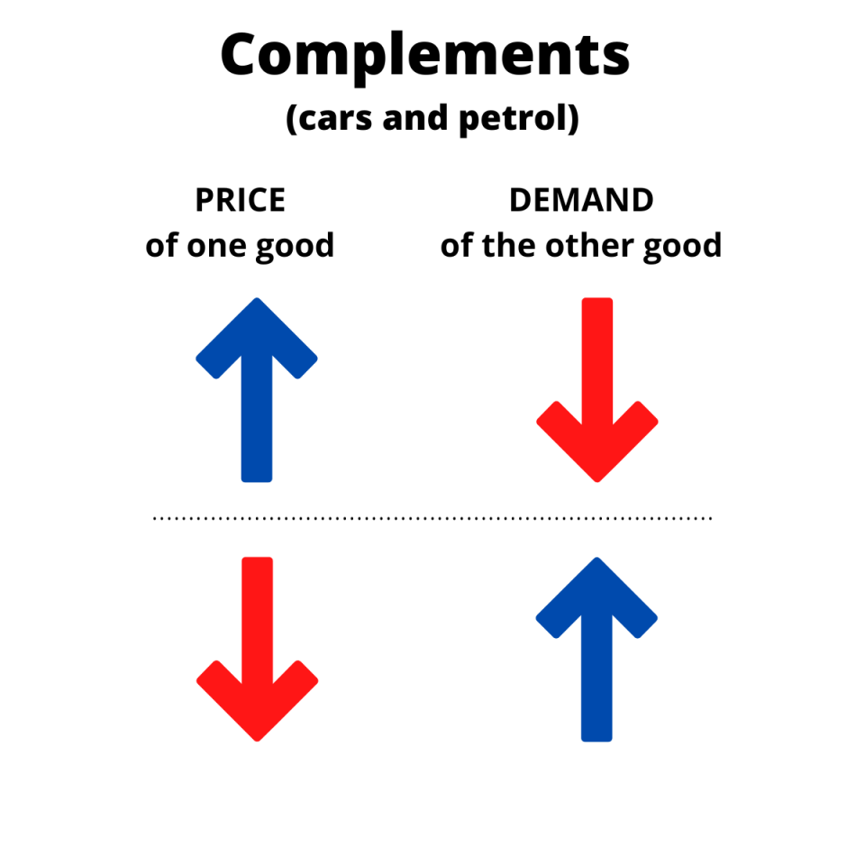
Therefore, the reduction in the price of one product, that is, a complementary good, will impact the D for the other product and shift the D curve to the right.
On the other hand, if the price of the good complementary increases, the D for the different products will decrease also, and the D curve will shift to the left. Examples of complementary goods are coffee & donuts, petrol, and cars.
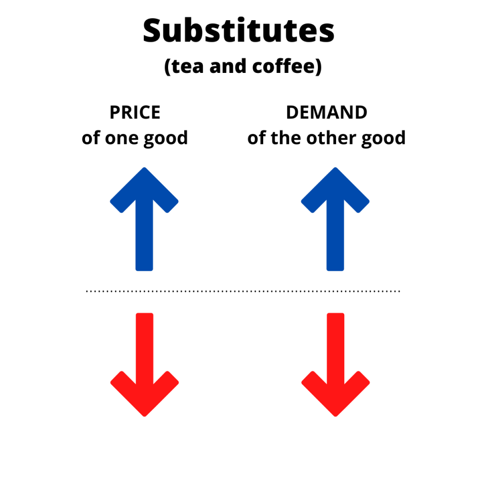
In the case of substitutes, those two goods could be easily exchanged for consumption. An example of reserves is water and soda or coffee and tea.
If the price of one substitute decreases, the D for the other good will fall, and the D curve will shift to the left. If the price of one substitute increases, the D for the other good will increase, and the D curve will go to the right.
Income
Increases and decreases in income influence demand, as it directly impacts consumption. However, for different kinds of goods, the changes in income have a different effect on consumption. We are talking here about two main types of goods:
- Normal goods
- Inferior goods.
For common goods, the D is growing with increased income. On the other hand, the D is declining with increased pay for inferior goods.
Some goods are also necessary, as people need to buy them regardless of their income level. On the other hand, people buy luxury goods only with a certain income. Therefore, for luxury goods, the increase in D is more than proportional to the rise in revenue.
Demographic Changes
The general rule here is that the higher the population, the higher the D. Also, some specific characteristics of the people will impact the D for certain products and services.
With the baby boom, there will be increased D for baby products. On the other hand, with the population altering, the D for medical services will grow.
Buyer Expectations
Buyers could have different expectations that will impact the D shifts. For example, if buyers expect that the price of certain goods will increase, they will buy more in the present.
Also, if there are expectations of any technological improvement of a particular product, the D for the old type will decrease.

What are the goods with an upward-sloping demand curve?
However, research also looks at the minority of goods and services in which price and quantity have a positive relationship in certain circumstances. For example, according to the Principles of Economics, the idea that goods can have an upward-sloping demand curve is attributed to Robert Giffen.
Therefore, goods that are inferior and have an income effect strong enough to overcome the substitution effect are called Giffen goods.
Also, Marshal mentioned Giffen's behavior in his Principles of Economics in 1895. However, later empirical research refuted the example of potatoes during the Irish starvation in 1845-49.
Several studies suggest that an upward-sloping D for goods can exist in certain circumstances. For example, the newest research indicates that rice in southern China can be Giffen good for impoverished consumers, while in northern China, it is noodles.
In their recent study, Robert Jensen and Nolan Miller explain Giffen behavior: Theory and Evidence (2007). As rice and noodles are the central part of Chinese cuisine, the purchases of the item represent a considerable percentage of their income.
Once the price of the rice and noodles increases, the poor consumers reduce consumption of other goods to buy their needed portion of rice and noodles. In this way, the poor can achieve the required caloric intake even when the prices of their staples increase.
However, this result is only valid for some poor people in China. The authors found strong evidence of Giffen's behavior for the researched group: consuming at least some substantial share (20%) of calories from other sources than rice.
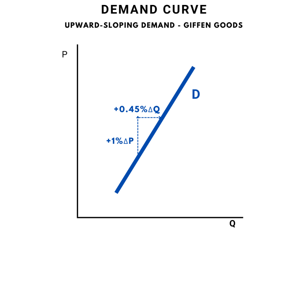
Those people belong to the category "the poor-but-not-too-poor," and it is valid that a one percent price increase causes a 0.45 percent increase in consumption.
For those households that consumed only rice, the price increase left them no choice but to decrease the bought quantity and therefore reduced their calorie intake.
An example of the upward-sloping D curve from Jensen's and Miller's research is illustrated below:
David McKenzie also tried to prove the existence of Giffen goods. In his study, Are tortillas a Giffen good in Mexico? (2002), he found out that tortillas are an inferior good for poor Mexicans.
However, the tortillas are not a Giffen good, most likely, due to the broader range of alternatives the poor Mexicans have compared to the poor Chinese consumers.
Demand: microeconomic Vs. macroeconomic
When discussing it in economic terms, it is necessary to distinguish between the microeconomic and macroeconomic views on demand. As stated in Samuelson and Nordhaus's classical textbook on Economics, macroeconomic or aggregate demand (AD) curves differ from their microeconomic cousins.
The mico curve (D) analyzes the behavior of an individual commodity. The macro curve (AD), on the other hand, reflects changes in prices and output for the entire economy.
According to the Principles of Economics, in the macroeconomic view, firms face four sources:
- Households (personal consumption)
- Other firms (Investment)
- Government agencies (government purchases)
- Foreign markets (net exports),
Aggregate demand (AD) is the relationship between the total quantity of goods and services demanded from all four sources of demand and the current price level (while all the other determinants of spending are unchanged).
In other words, the AD is the total or aggregate quantity of output bought at the given level of prices in the economy. The components of AD are equivalent to the parts of the full national work measured as the gross domestic product (GDP).
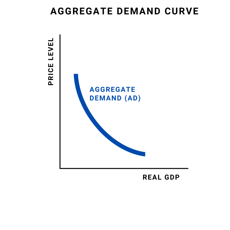
In addition, the AD curve slopes downwards similarly to the microeconomic demand. However, the downward slope is not caused by the same effects. The slope of the AD curve is two reasons:
Those reasons differ from the microeconomics version of the demand curve D, which slopes downwards because of the substitution effect and income effect.
It is also important to note the alignment of the four sources of AD and four components of the GDP. According to the expenditure approach for estimating the output, the five main categories of expenditures are considered:
- Consumption (C)
- Investment (I)
- Government purchases (G)
- Net export (Export-Import) X


or Want to Sign up with your social account?