SEARCH Function
It is categorized as a text function that returns the position of a substring or a character inside another text string.


What is the SEARCH Function?
The SEARCH function in Excel is like using the search bar on your computer. When you're looking for a file, you type its name, hit Enter, and your computer tells you where it is. In Excel, the SEARCH Function does a similar job—it looks for something in a collection of items and returns its position to the user.
That "something" is usually a text string or a character inside another text string. The function is rarely used on its own and is usually combined with other text functions such as LEFT, RIGHT, or MID to extract particular characters or text strings.
This article will explain the syntax for the function and provide examples of how you can use the function to extract data from a string of characters.
Key Takeaways
- The SEARCH function locates a substring or character in a text string, similar to the Windows search bar, and is often used with other text functions to extract specific data.
- The inputs are find_text, within_text, and optional start_num. Notably, SEARCH is case-insensitive and allows wildcard characters, distinguishing it from FIND.
- It can be combined with ISNUMBER to check if a substring exists in data. Useful for tasks like verifying email domains.
- It can be used to perform complex text extraction for first, middle, and last names using SEARCH, LEFT, MID, and RIGHT functions.
understanding The SEARCH Function
SEARCH is categorized as a text function that returns the position of a substring or a character inside another text string.
For example, if you have the text string as 'Walmart Inc is the biggest retailer in the world" and you need to find the position of "retailer" in the text string, then the function will give an output of 28.
The function counts the number of characters from the left-hand side and returns the position corresponding to the substring's first character.
The result that we get is for the position of 'r' in our substring 'retailer' as 28. Using the function in combination with other text functions, you can extract a particular substring as a result while ignoring the rest of the characters in a text string.
The function is very similar to the FIND function, which also returns the position of a substring in another text string. The major difference is that SEARCH is not case-sensitive, and allows the use of wildcard characters.
For example, if you have the text string as 'Amazon Inc' and ask the function to find the position of 'A' or 'a' in the text string with a starting position of 1, it will return the result as capital 'A' for both the inputs.
Since the function isn't case-sensitive, it does not matter whether the substring is capitalized or in lowercase.
Similarly, if you use wildcards to find a substring, the function will be able to return the required result based on the potential searches that it finds in the text string.
The syntax for the SEARCH function
The syntax for the function is:
=SEARCH(find_text, within_text, [start_num])
where,
- find_text = (required) the substring that we intend to search for in the text string
- within_text = (required) the text string which will be searched for the substring.
- start_num = (optional) the starting position within the text string to search for the substring. For example, suppose that you have the text string as 'Jeff Bezos' and need to find the position for 'e' in the first name. If you input the default value of 1, the position for the substring will be 2.
If the start_num is equal to 5 (the space character), then the position for the substring becomes seven which skips the 'e' in the first name and returns the position for the character 'e' in the last name.
Thus the start_num argument can be beneficial if you intend to skip a similar substring and return a different substring from the text string.
How to use the SEARCH Function in Excel?
The function can either be used from the Functions library or written into the worksheet as a formula. We will explore both the methods on how to use the function below:
a) Method #1: From the Functions Library
Functions are predetermined formulas where you just need to input the arguments and directly get the result in the selected cell. To use the function from the function's library, please follow the below steps:
1. First, select the cell in which you intend to return the result.
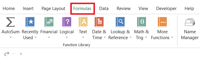
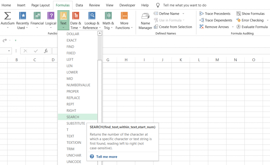
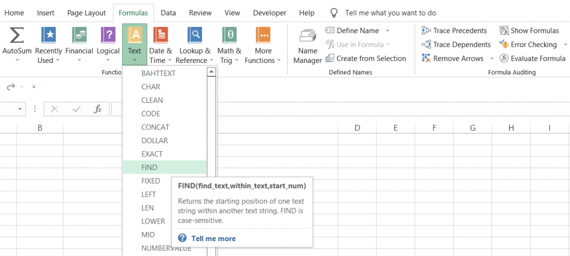
2. Click on the Formulas tab > Text drop-down in the function's library and select the SEARCH function.
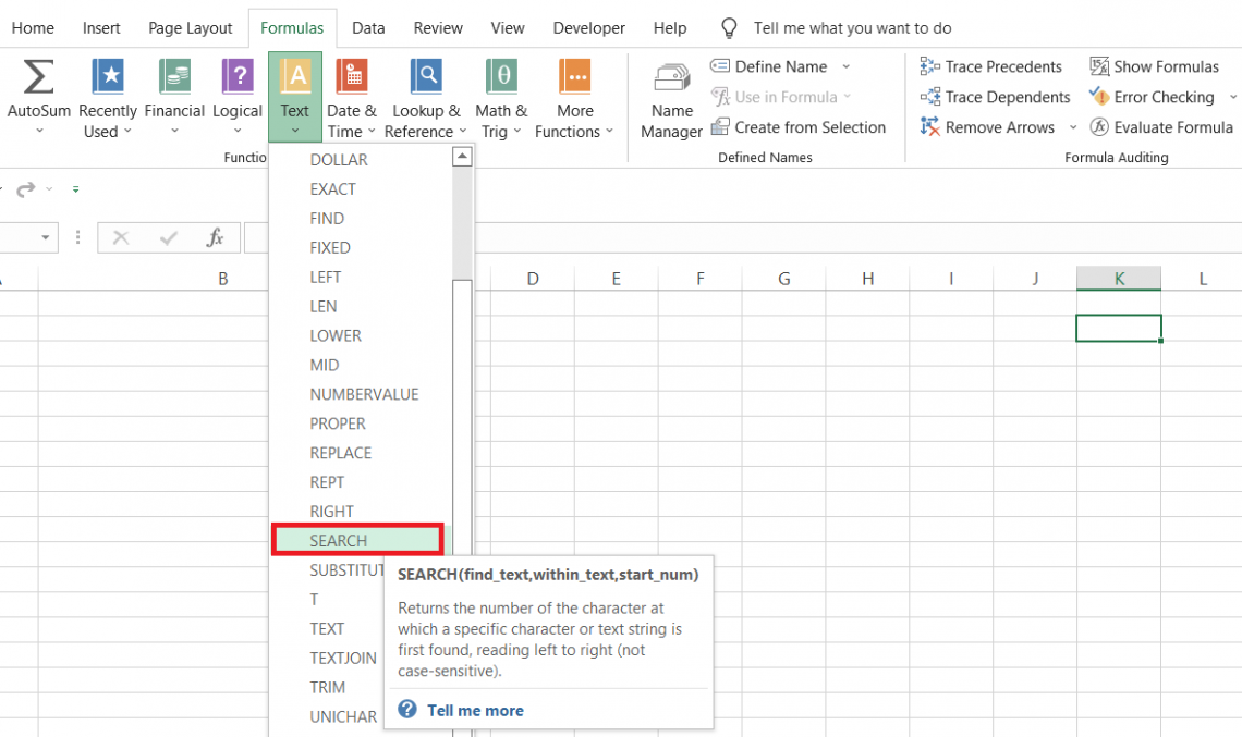
3. This will open up the function dialogue box as illustrated below:
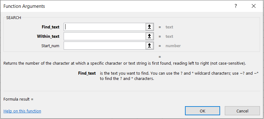
4. Input all the parameters in the respective text boxes as per the syntax of the function. For example, we have input the below data in the respective boxes.
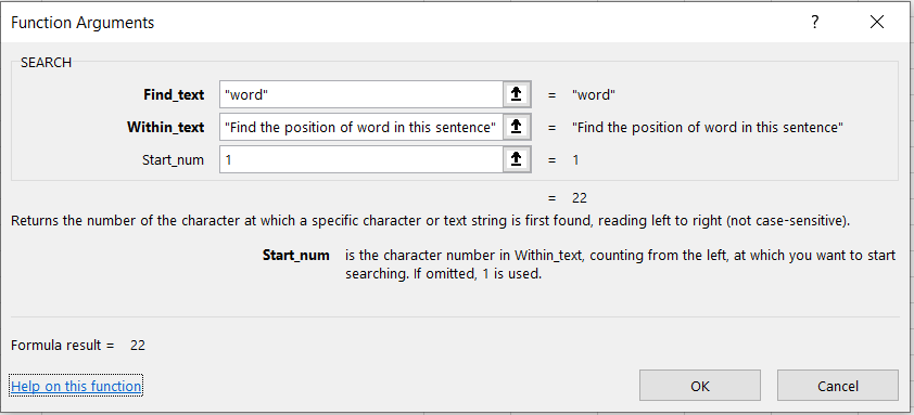
5. Click on "OK." This will give you the result in the selected cell as illustrated below:
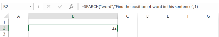
6. Since ‘w’ is the first letter of the substring ‘word’, we get the position that corresponds to the letter which is 22.
7. As our start_num was equal to 1, the function counts the characters beginning from the left-hand side.
b. Method #2: As a Worksheet formula
To use the function as a worksheet formula, you begin with an equal sign and input the formula name followed by the arguments in the function.
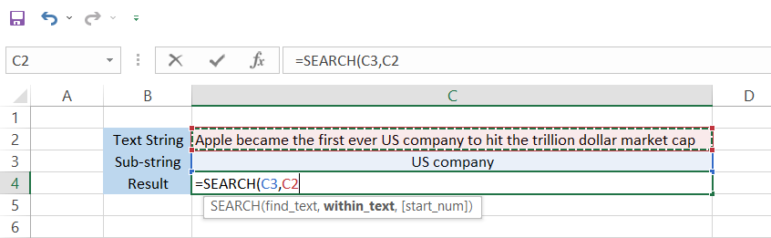
Suppose that you have the data in Excel, as illustrated below:
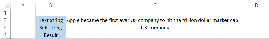
1. find_text - The text we intend to find is in cell C3. The formula becomes =SEARCH(C3, within text,[start_num])
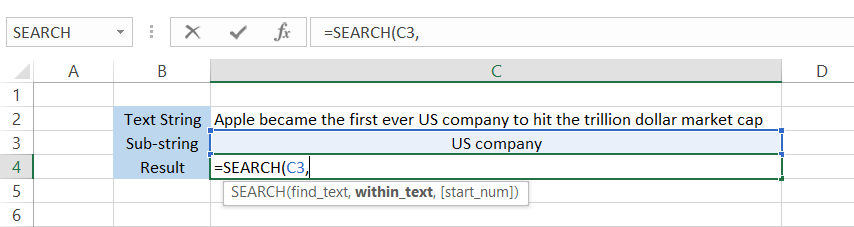
2. within_text - Next, we reference the cell in which we need to search for the sub-string. i.e., cell C2. The formula becomes =SEARCH(C3,C2,[start_num]) as below:
3. start_num - Since this argument is optional, you can skip it and press Enter. If you skip the value the argument takes in a default value of 1. However, to be precise we will input 1 into the parentheses.
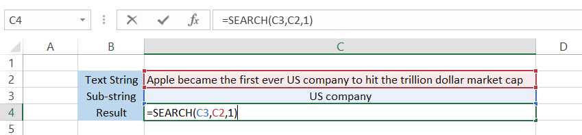
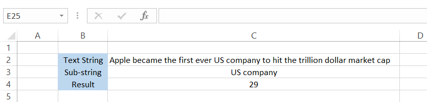
Finally, all you need to do is press Enter, and the formula will give you the result as 29.
Applications of the SEARCH Function
Since we have already seen how the function works above, we can combine it with different compatible functions to show just how useful it can be.
a. Checking for the presence of a substring
If you just need to check whether a particular substring exists in the data, you can use the ISNUMBER and SEARCH function combination.
We already know that the function will return the position of a substring as a numerical value.
When you pass this numerical value through the ISNUMBER function, it will evaluate to TRUE, whereas if it's not a number, it will return a result of FALSE.
Suppose that you have email addresses as illustrated below:
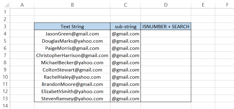
Suppose you need to check which email addresses have the domain @gmail.com. For this, you will use the formula =ISNUMBER(SEARCH(C4, B4,1)) in cell D4.
As we haven't used the dollar sign($) to freeze the rows or columns, the formula would automatically accommodate the corresponding cell addresses formula once you drag it down.
When you input the formula in all the cells up to D13, we get the following result:
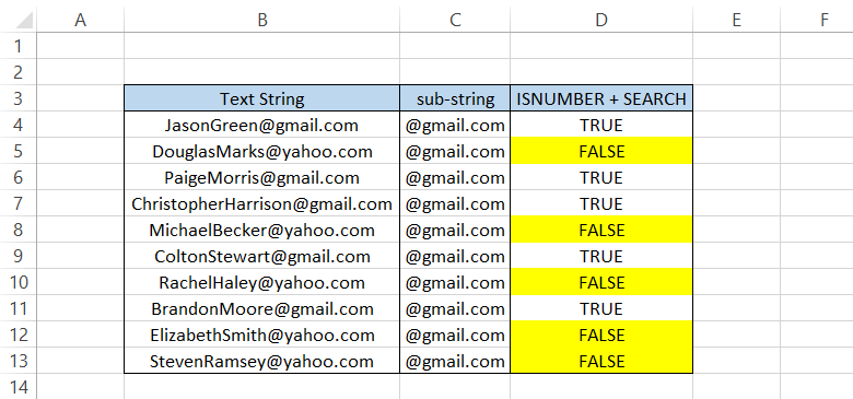
The FALSE results mean that the respective email addresses don't have the domain @gmail.com.
b. Separating first and last names
A lot of times, you would find the need to separate text into two or two different text strings, especially full names.
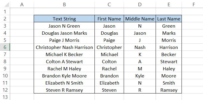
Suppose that you have the list of names below:
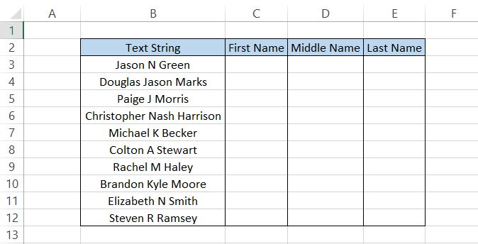
Before we use the formula, remember that "represents space character between the quotation marks as you might see these characters many times in the formula!
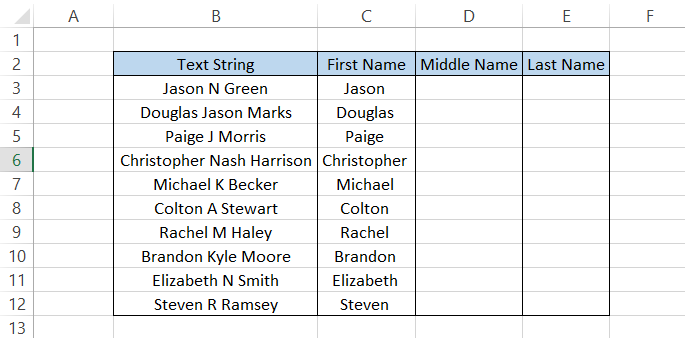
To extract the first name, we will use the combination of the LEFT and SEARCH functions. The formula used will be =LEFT(B3, SEARCH(", "B3,1)), which will give you the result shown below:
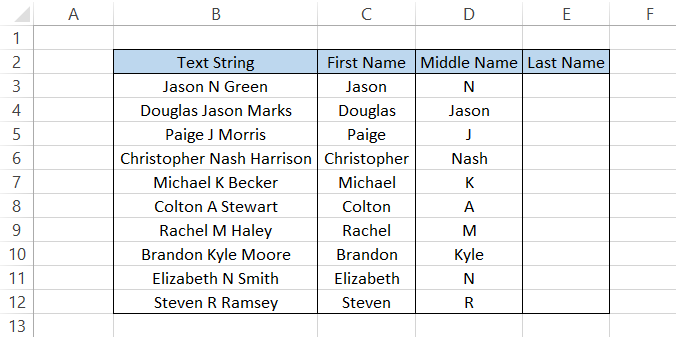
The middle names will be extracted using the formula =MID(B3,SEARCH(" ",B3)+1,SEARCH(" ",B3,SEARCH(" ",B3)+1)-SEARCH(" ",B3)-1) which should give you the result in column D as:
Complicated formula? Let's try to break it down to understand it better.
The MID function has three arguments - text to extract from(B3), starting position to extract(SEARCH(“ “,B3)+1 and the number of characters to extract(SEARCH(“ “,B3,SEARCH(“ “,B3)+1)-SEARCH(“ “,B3)-1)
- The B3 is simply the text we want to extract from, i.e., Douglas Jason Marks.
- The SEARCH(", "B3)+1 finds the position of the first space character in the text string. By adding a 1, we skip the space character and begin the extraction from the first character of the middle name. For example, 'J' in Jason as in cell B4
- The tricky part of the formula is SEARCH("",B3,SEARCH("",B3)+1)-SEARCH("",B3)-1.
Here, we extract the 'n' number of characters. In simple terms, this part of the formula takes the first letter of the middle name as the first character to extract.
The result of the formula behind the scenes is 'Jason Marks.' On this exact same text string, the result of the final part of the formula -SEARCH(", "B3)-1 runs which finds the space character after the middle name.
One character subtracted from the formula gives us the final result as 'Jason' in cell D4. Even though the function does all the hard work, we don't have to forget that the extraction is only possible with the outermost MID function in the formula.
The middle name is separated by a delimiter 'space' character which enables us to use the function to find those 'space' characters and thus extract the middle name.
Delimiters serve to separate chunks of data. These can be spaces, commas, semi-colons, etc.
Finally, you can obtain the last name by using the formula
=RIGHT(B3,LEN(B3)-SEARCH(" ",B3,SEARCH(" ",B3,SEARCH(" ",B3)+1)))
which will give you the following result:
C. Extracting text from between different delimiters
When you receive a file from a third party, chances are there might be many irregularities in the data. For example, sometimes, a delimiter might exist in your data that may disrupt the flow of data.
To extract the data between these delimiters, you can use MID and SEARCH functions.
Suppose that you have the data illustrated below:
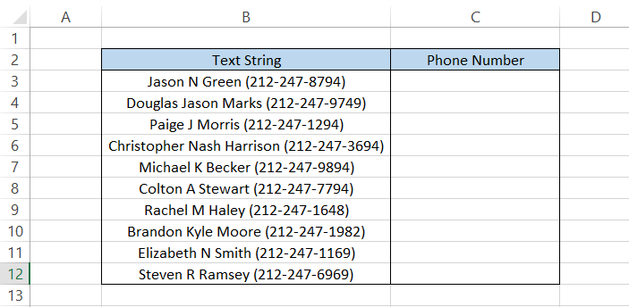
The phone numbers are separated by delimiters in the form of parentheses "( )".
To extract the phone numbers, we will use the formula
=MID(B3,SEARCH("(",B3)+1,(SEARCH(")",B3))-SEARCH("(",B3)-1)
which will give you the following results:
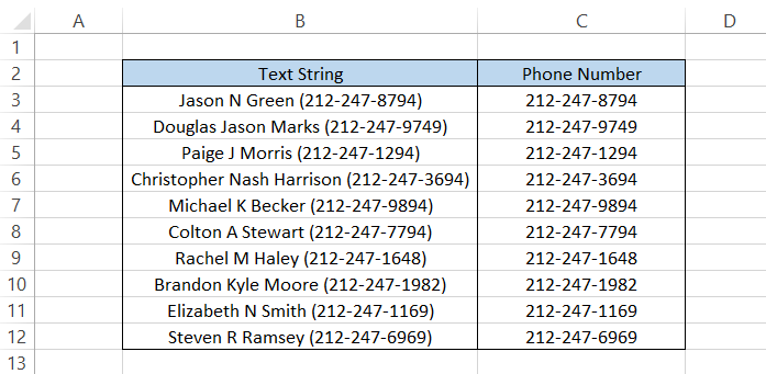
Parentheses are a delimiter where both have different symbols, i.e., left and right parentheses. But what if you have two similar delimiters?
If you have a different delimiter, say a number sign (#), in place of parentheses, you can use the formula:
=SUBSTITUTE(MID(B3,SEARCH("#",B3)+1,SEARCH("#",B3)),"#","")
which will give you the result as illustrated as below:
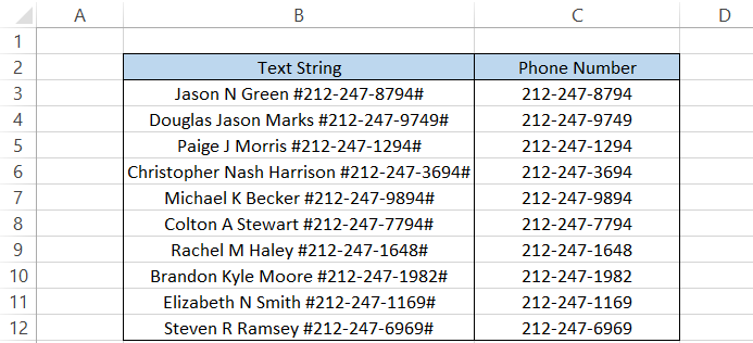
Note
The formula works for all the symbols except the wildcard characters, such as the apostrophe(*) and question mark(?).
SEARCH vs. FIND function
FIND is categorized as a text function. It finds a substring and returns its relative position in a text string.
Both functions work similarly. The only major difference in the FIND function is that it is case-sensitive.
For example, if you need to find 'a' in 'Apple', then the function will return an error. On the other hand, if you try to find 'A' in 'Apple,' the FIND function will return the character's position as 1.
The syntax for the function is:
=FIND(find_text, within_text, [start_num])
find_text = (required) the substring that we intend to find in the text string
within_text = (required) the text string which will be searched for the substring
start_num = (optional) the starting position within the text string to search for the substring
To see the difference between both functions, we will see an example. It is entirely up to you what function you prefer since each one has its pros and cons.
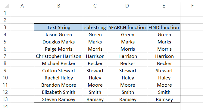
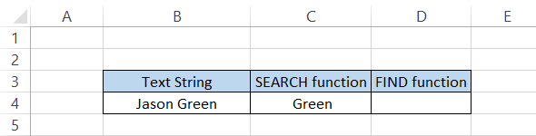
Suppose you have the full names in column B, as illustrated below:
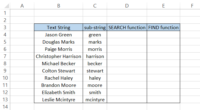
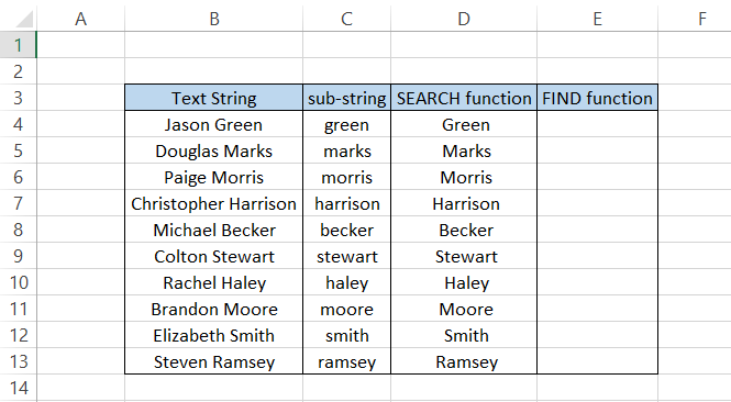
We need to extract the last names using the substrings in column C. The formula to extract the surname in cell D4 will be =MID(B4,SEARCH(" ",B4,1),SEARCH(C4,B4)). After dragging the formula down up to cell C13, we will get this result:
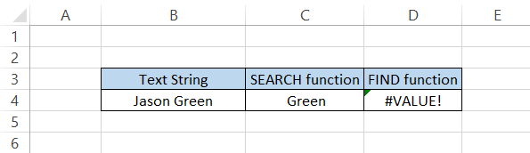
A similar formula can be used where FIND will replace SEARCH. The updated formula becomes =MID(B4,FIND(" ",B4,1),FIND(C4,B4)) which will give you a result of #VALUE! error.
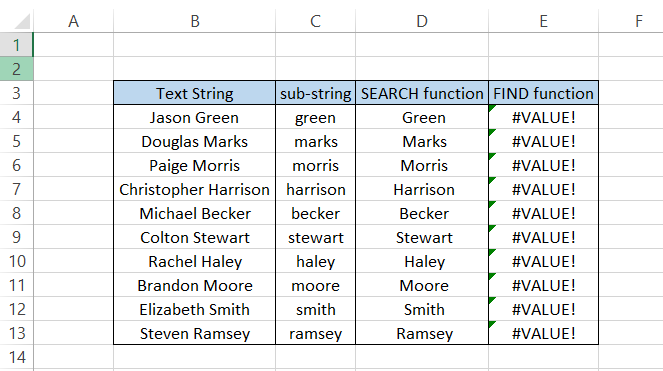
Hmm, something is wrong. As we can recall, the FIND function is case-sensitive. Moreover, all of our sub-strings begin in lowercase letters, whereas the last names in column B begin with capital letters.
If we change the sub-strings to last names beginning with capital letters, the function is finally able to return the result that we expect.
On the other hand, there is no issue when you use the SEARCH function. This can be an advantage as well as a disadvantage to the user.
When you specifically want to find an exact substring, FIND is the best function to use. However, if you do not have any need to find an exact match, then the SEARCH function works wonders.
Another reason the FIND function is inferior is that it cannot find substrings using wildcard characters.
By using just a part of the substring followed by an asterisk(*) wildcard character, the SEARCH function can accurately return the desired result, whereas the FIND function returns a #VALUE error.
The formula used to return the result with wildcard characters is =MID(B4,SEARCH(" ",B4,1),SEARCH("Gre*",B4)) which will give you the following result:
Whereas a similar formula =MID(B4,FIND(" ",B4,1),FIND("Gre*",B4)) replaced with FIND function will give the #VALUE! error.
As stated above, the FIND function does not accept wildcards along with substrings "Gre" to find the word "Green" in the text string. This is why sometimes the SEARCH function is superior to the FIND function.

Researched and authored by Akash Bagul | LinkedIn
Free Resources
To continue learning and advancing your career, check out these additional helpful WSO resources:

or Want to Sign up with your social account?