#REF Excel
A message Excel displays when a formula references a cell that no longer exists


What are #REF Excel Errors?
You might have faced countless instances when you use the VLOOKUP or other formulas in Excel and you received the #REF! Error instead of the expected result the next time you open the file. This error usually occurs when the reference used in the formula is invalid.
When you add a new column in the middle of the spreadsheet or delete that empty row, it changes the reference used in the formula. Additionally copying the formula from one cell to another can cause reference errors.
Key Takeaways
- The #REF! error in Excel occurs when a formula references an invalid cell or range, typically due to changes in the structure of the spreadsheet such as deleting rows or columns used in the formula.
- To avoid #REF! errors, it is advisable to make structural changes to the spreadsheet before referencing the data, maintain duplicate sheets or workbooks, and freeze cells when copying formulas to new cells.
- Finding and correcting #REF! errors can be done efficiently using methods like the 'Go to Special' function, conditional formatting, and the Find and Replace tool.
- Precautionary measures can prevent #REF! errors in Excel, highlighting the importance of planning and careful management of data references in formulas to maintain data integrity.
Understanding #REF Excel Errors
A #REF! Error usually occurs when Excel is unable to understand the cell or the range reference made in the formula. This happens when you delete a certain row or column that has already been used in the formula.
For example, let's say that you use VLOOKUP on an Excel workbook A and pull in values from Excel workbook B. If you accidently delete column E in workbook B, it will cause a cascade effect and give you a #REF! Error for all the values starting from column E until the end next time you open the workbook A.
Since the reference for the formula is deleted, i.e., the E column, Excel is unable to understand what value to pull in at that instance. As a result, we see the #REF! Error as an Excel's way of saying that the reference is invalid.
#REF Excel Error Example
Suppose that you buy certain stocks for your portfolio starting from 2nd Feb 2022 until 15th Feb 2022. You note down the transactions in a Excel file that looks as below:
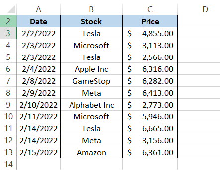
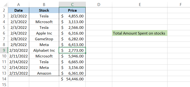
You use the AutoSum function using the Alt + equal sign (=) in cell C14, i.e., =SUM(C3:C13) and get the result as $54,446.00 which is the total amount spent on buying stocks for your portfolio. However, you want the sum in the F6 cell so as to make it easily accessible to link it to other spreadsheets and review it on a daily basis.
You copy the formula using the Ctrl + C and paste it in the cell F6 using the Ctrl + V only to get the #REF! Error.
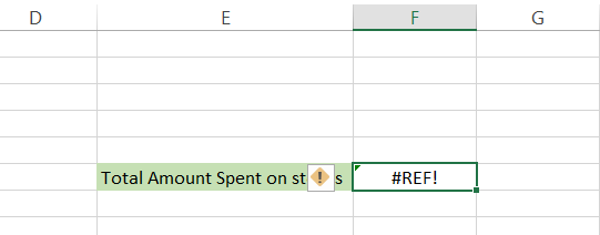
This is because previously our SUM formula had 11 cells in the reference above it but after copying the formula in cell F6, there exist only 5 cells above the formula. This confuses Excel which then gives you the error.
How to avoid #REF Excel Error?
“Prevention is better than the cure.” If seeing the #REF! Error frustrates or makes you sick in the stomach (well,that's too much), we suggest that you make sure to stop them from occurring in the first place.
- If you need to delete a certain row or column, do it before you reference the data in the formula. That way the cells or range you refer to in the formula remain intact.
- Always make sure to have the duplicate sheets or workbook for the data. If any of the data gets misplaced and causes an error, you can easily overwrite it to the original data.
- When you copy the formula to a new cell, freeze the cells using F4 such that C2 becomes $C$2 to avoid the #REF! error.
- Just in case if you accidentally delete a row/column, you can press the keyboard shortcut of Ctrl + Z to undo the error.
- If you wish to avoid the reference errors caused by VLOOKUP/HLOOKUP then use INDEX-MATCH function or the XLOOKUP function as the alternatives.
No, this section of the article is not a WikiHow or Dummies-101 but rather advises precautionary measures to prevent such errors. After all, it's better to sail on still waters rather than in stormy weather.
How to Find #REF Excel Errors
The reference errors can be quite obvious when it's just one cell where the value is expected as in our earlier example. But what if your spreadsheet consists of hundreds or thousands of rows of data and you need to figure out all the reference errors in the spreadsheet without manually going through them. There are two ways in general by which you can locate and clear the #REF! Error.
Method #1: Go to Special function
If you need to find specific cells based on formulas, blank, logics or errors in your spreadsheet, you should ‘Go to’ the Home tab and select the Go to Special function that you will find under the Find & Select.
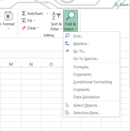
The Go to Special function basically lets you to find all the cells that meet a particular criteria such as #REF! Errors. You can also access this function by using the keyboard shortcut of either F5 or Ctrl + G followed by Alt + S which opens up the following dialog box:
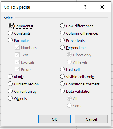
Select the radio box for Formulas or use keyboard shortcut Alt + F and untick all the options, i.e., Numbers, Text, Logicals except Errors. Click on OK. So, if you have multiple #REF! Errors in your spreadsheet, it will select all those cells as shown below:
This method is useful if you just need to find the errors so you can tackle them individually if they have different references and logics set up in them.
Method #2: Conditional formatting
Conditional formatting has to be one of the most underrated functions in Excel. Most analysts keep boasting about how they used multiple nested IF statements to build extremely dynamic financial models but undervalue conditional formatting function due to its simplicity.
To use conditional formatting, first select the entire spreadsheet using the Ctrl +A or highlight the specific table in which you need to check the errors. Click on the Home tab and then onto Conditional Formatting which you will find in the Styles section. Navigate and click on the ‘New Rules’ option.
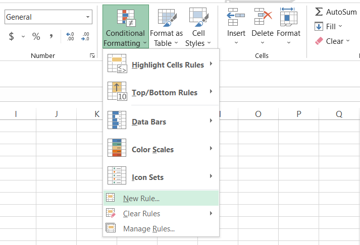
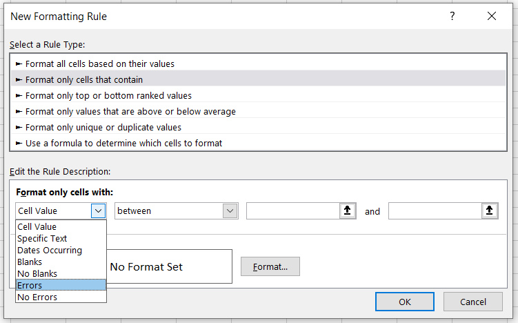
This opens a ‘New Formatting Rule’ dialog box where you need to select the rule type as ‘Format only cells that contain’. Next, you will get an option to Edit the Rule description where you need to select ‘Errors’ from the drop down menu to format the specific desired cells which in our case are the reference errors.
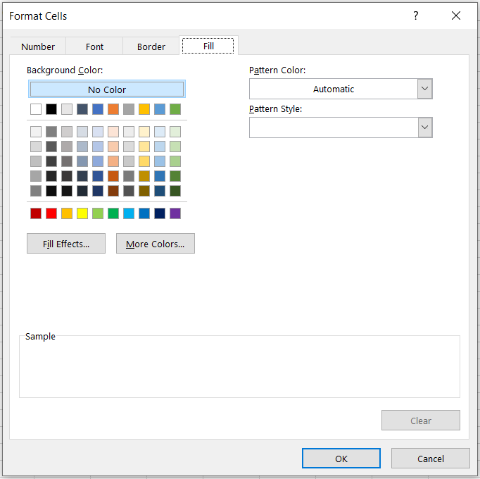
Select the desired fill color by clicking on the Format button and then selecting the Fill tab in the subsequent Format Cells dialog box and press OK.
When you finally press OK in the New Formatting Rule dialog box of conditional formatting, the result you will get from the apparent logic set up is as:
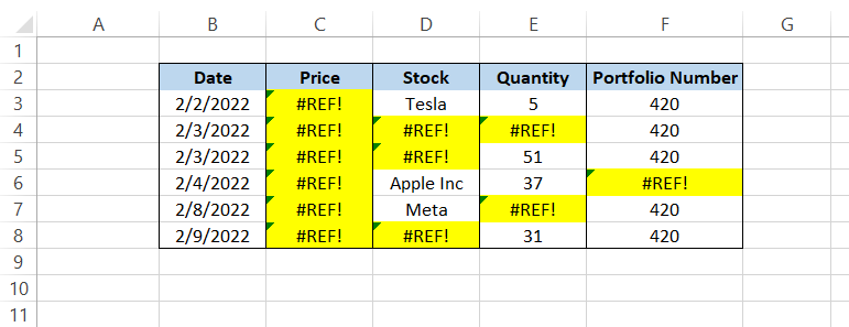
This approach goes one step ahead than the Go to Special function by highlighting the cells containing errors rather than just selecting them and doing nothing.
Method #3: Find and Replace
A more efficient approach than either Go to Special or Conditional formatting in finding as well as replacing the errors is the Find and Replace function of Excel.
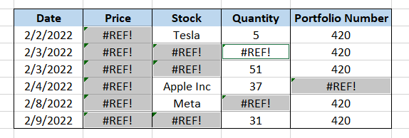
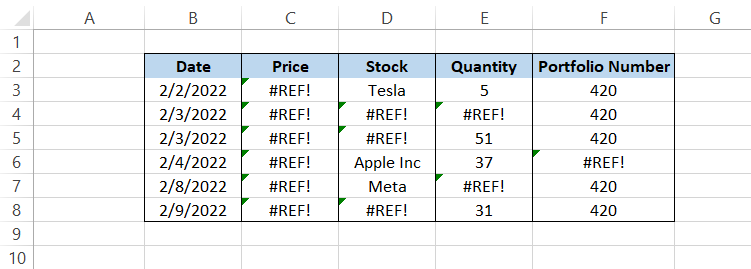
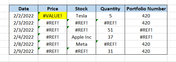
Most of the time, if you know what is causing the reference error, you can just manually fix it by changing the reference used. However, if you are not sure what has caused the error, it's best to leave those cells blank. This can be achieved with the help of Find and Replace function. In the table below we can find several #REF! errors:
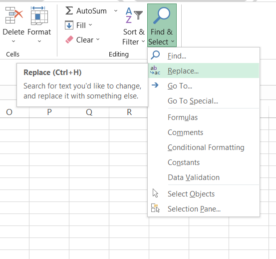
Click on the Home tab and select the Replace function that you will find under the Find & Select.
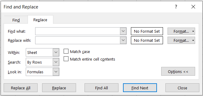
Alternatively, you can also use the keyboard shortcut of Ctrl + H to open the Find and Replace dialog box. If you just need to find the errors or any specific value in the spreadsheet, click on the ‘Find’ tab. By clicking on the ‘Replace’ tab, you can find a specific value or error in the spreadsheet and replace it with a desired value such as zero or empty strings.
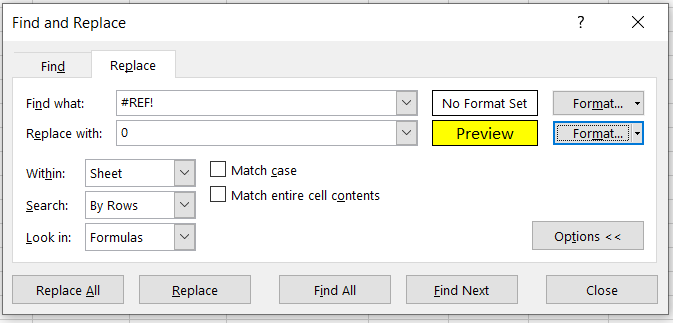
Now to use this function set your ‘Find what’ value as #REF! Error while the Replace with value will be zero. Additionally, you can format your replace values with different font, font size, cell fill colors from the Format option.
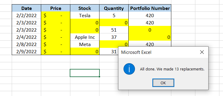
You have two options now: Iterate through all the reference errors by replacing them with 0 using the ‘Replace’ option or Replace them all in one go. When you click on ‘Replace All’, Excel displays a message that says the replacements are done. As we had also set the fill color for the cells, whatever cell values were replaced by zero, were highlighted with yellow color.
Important Note: The reason we have replaced the reference error with zero is to avoid the #VALUE! error. If you replace the #REF! Error caused by a formula with a text, Excel throws another error in form of #VALUE!.
As you can see, our formula becomes =SUM(#REF!) after the reference error, so the find and replace tool just replaces the value inside the brackets with the text or empty string. That means the formula becomes =SUM(“”) or =SUM(Error).
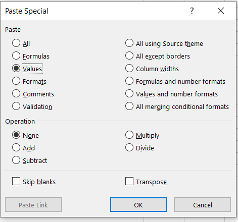
To avoid this, it's best to replace it with zero or if feasible paste the formulas as values to replace them with whatever value you would like. To paste formulas as values, use keyboard shortcut of Ctrl + C by copying the entire range and then overwrite the copied data by using keyboard shortcut of Ctrl + Alt + V to select the radio box for values.
Method #4: IFERROR formula
This might not be the best approach while dealing with reference errors but nevertheless makes it a great tool to highlight them. The IFERROR function returns a particular value that is specified in the formula if the parameters returns #N/A, #VALUE!, #REF!, #DIV/0!, #NUM!, #NAME?, or #NULL! Errors.
The syntax for IFERROR function is:
=IFERROR(value,value_if_error)
where,
- value = A required parameter that is checked for an error
- value_if_error = Particular value/text expression that is returned if formula finds error in ‘value’ parameter.
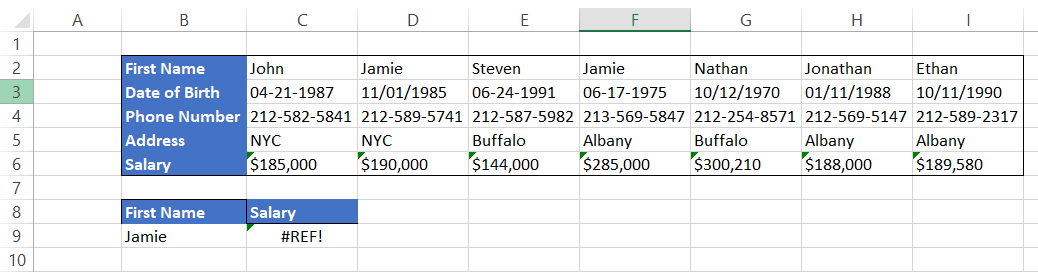
Let's say that you need to find the Salary for Jason from the horizontally oriented table.
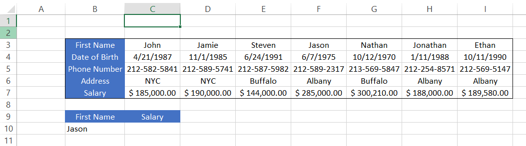
You use the HLOOKUP function along with the IFERROR so that your formula becomes =IFERROR(HLOOKUP(B10, C3:I7, 6, FALSE), "Error!"). This means that if VLOOKUP cannot find the reference for the value, the value that will be returned is Error!
As you can see, our table has a total of 5 fives but we have selected row_index_number as 6 in the formula. Such mistakes can happen quite often while working on extremely large data. The result that you will get in the cell C10 using the formula will be:
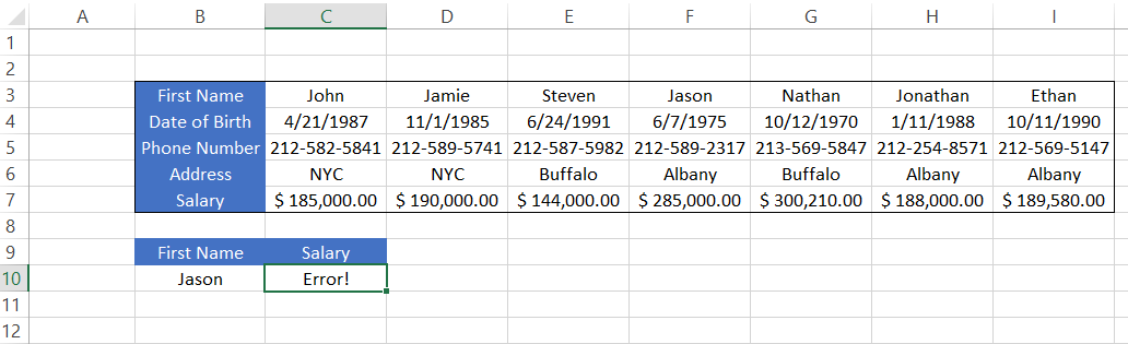
The only drawback to using this method is that it does not distinguish between different errors. Sometimes you might get an error other than for reference such as #DIV/0! which is due to a value being divided by zero. Addressing every error, in the same way, can be quite dangerous as it may affect the integrity of the data.
Hence, we can only wait and hope that Microsoft comes up with a dedicated IFREF function in Excel that gives a particular result if reference errors are encountered.

More on Excel
To continue your journey towards becoming an Excel wizard, check out these additional helpful WSO resources.

or Want to Sign up with your social account?