Advanced Excel Formulas
Inbuilt functions that aren't used on a day-to-day basis but are utilized to retrieve specific data from an existing dataset, perform complex calculations, and analyze data.


What Are Advanced Excel Formula?
Advanced Excel formulas are inbuilt functions that aren't used on a day-to-day basis but are utilized to retrieve specific data from an existing dataset, perform complex calculations, and analyze data.

Big Data has changed how most financial institutions work in today’s age of innovation. It plays a large role in finance, where it refers to large amounts of related data whose analysis produces actionable insight and makes it easier for investors to make better investment decisions. Excel enables the user to cope with the big data scenario consisting of the three H’s—high volume, high velocity, and high variety. It also makes data capture and processing more manageable, making exploratory and ad hoc data analysis favorable.
Based on many years of experience, we have compiled the ten most important and advanced Excel formulas that every world-class financial analyst must know. These functions can help shave minutes off your work and make the overall Excel worksheet more fleshed out and connected. While it may not sound like much, these minutes can eventually add up to hours of saved work.
Below is the countdown of the most advanced and helpful Excel formulas to take your modeling skills to the next level.
10. INDEX MATCH
INDEX MATCH is one of the most essential Excel functions. It is a combination of two functions that are almost always used together. This advanced function searches for a particular value(s) in a list and returns the relative position of that value in the list. It allows the user to create two-way lookups, left lookups, case-sensitive lookups, and even lookups based on different criteria assigned by the user.
Unlike VLOOKUP (which can use the value from only the first column), it lets you use the lookup value from any column. Furthermore, VLOOKUP can be slower as it returns an exact value, while INDEX MATCH only returns a reference value.
For example, to find the hobby for “Jim” in column D, one would use INDEX MATCH with the following formula:
=INDEX(D3:D5, MATCH("Jim", C3:C5))
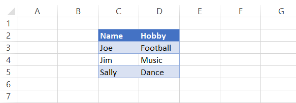
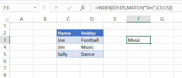
Here, the MATCH function looks for the value, and then the INDEX function returns the relative position of that value, which is “Music” in this case.
9. IF combined with AND/OR
The IF formula allows the user to make logical comparisons between two different values and returns a value based on the comparison result, i.e., different values for TRUE and FALSE outcomes. However, sometimes the data parameters can be numerous, generating a need for more than one IF function to test the various conditions and the result they return. During such instances, nested-IF statements can increase the number of feasible outcomes.
It can be used in conjunction with AND/OR where AND/OR test multiple conditions to return specific values based on the fulfillment of conditions. For example, consider the marks of subjects English and Math for fifth grade students. To progress to the next grade, the students must pass both subjects. The passing mark for both papers is 35. We can check whether the students passed by using IF in conjunction with AND.
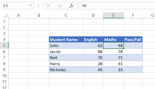
In this case, we will use the following formula to check if the condition of 35 marks is fulfilled for both subjects.
=IF(AND(D5>35, E5>35), “PASS”, “FAIL”)
We get the results as:
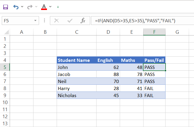
We see that since Harry and Nicholas both have received marks below 35 in English and Maths, respectively, they will not progress to the next grade.
Let’s assume that a new principal takes over the school administration who feels that obtaining the passing grade in both subjects is too harsh for the students. Therefore, they decide that students can progress to the next grade if they get passing marks in either of the subjects. This means that a student scoring above 35 in English OR Maths will advance to the next grade. This brings us to the following combination: IF with OR. We will use the following formula to check the pass and fail status.
=IF(OR(D5>35, E5>35), “PASS”, “FAIL”)
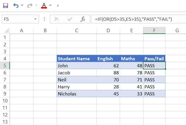
Now we see that all the students pass the exam and progress onto the next grade (Yay!).

8. OFFSET combined with SUM or AVERAGE
This is a beneficial formula that lets you do some powerful analysis in Excel.
The OFFSET function lets you create a new range starting at any cell or row, based on the number of rows and columns to offset, and the SUM or AVERAGE functions operate on all of the cells in that new range, respectively.
This means if you want to summarize your data by column (or row) but don’t know how many columns (or rows) there are, you can use this formula to find out the sum or average of your data.
Let’s say you want to find the total amount of revenue generated from an online store for the first ten days. You have several lines of data for each item sold, as shown below:
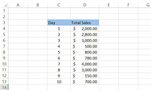
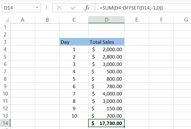
You can create a dynamic formula using the combination of SUM and OFFSET. Then, whenever you add a new line of revenue data, the formula will automatically calculate the total revenue up to the recent date. Below is the formula that will give you the dynamic sum.
=SUM(D4:OFFSET(D14, -1, 0))
Suppose we add the total sales data for Day 11. Then, we simply insert a row below day 10 and add the sales value as $2,000. You will notice that your formula automatically captures the latest value and gives you the updated sum of the total sales.
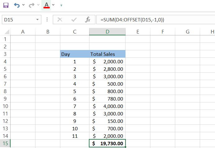
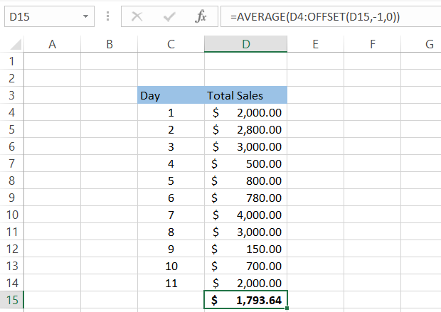
Similarly, you can use the AVERAGE() function to determine the average sales done up to the recent date or a single month. For example, the following formula will give you the average value of sales done up to the recent period.
=AVERAGE(D4:OFFSET(D15,-1,0))
7. CHOOSE
CHOOSE is a useful function for when you want to pick a value from a list of possibilities. You can use CHOOSE when you need to enter an option in Excel, and the user can select from a list of choices. For instance, it is often used in survey type questionnaires when you want people to answer with one of three possible answers.
The syntax for CHOOSE is given below.
=CHOOSE(index,value1,value2,...)
Here, index is a number between 1 and the total number of values.
For example, please consider the following list.
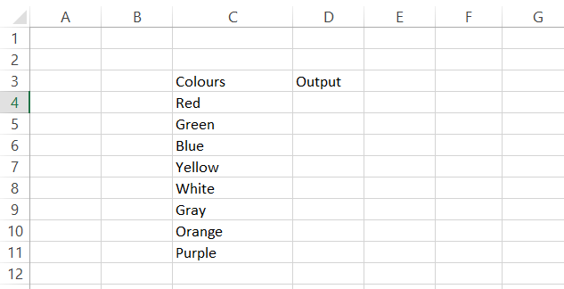
If you type “CHOOSE(2)”, it will return “Green,” and if you enter “CHOOSE(5)”, it will return “White.”
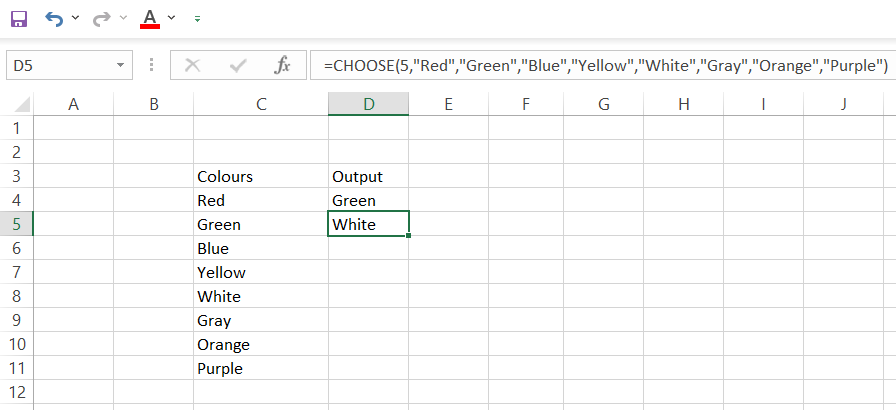
Note: The CHOOSE function can include reference values but will fail to retrieve values from a range or array constant. For example, the below formula will return “White.”
=CHOOSE(5, C4, C5, C6, C7, C8, C9, C10, C11)
But, if you use the following formula, it will throw the #VALUE error.
=CHOOSE(5, C4:C11)
This function is perfect for when you have lots of data listed in order. In addition, you can use this function to pick numbers for graphs and other calculations.
6. XNPV and XIRR
XNPV calculates net present value, which takes the future cash flow into account and calculates how much that cash flow is worth today, while XIRR calculates internal rate of return, which calculates the rate of return on an investment based on its cash flows. As opposed to the IRR function, which assumes that the cash flows occur at regular intervals, the XIRR function considers the dates when the cash flows occur, making it easier to calculate the actual internal rate of return for nonperiodic cash flows.
XNPV and XIRR are closely related formulas since the internal rate of return is the discount rate in DCF analysis that makes the net present value of all cash flows equal to zero. Hence, these are essential formulas to have at your disposal because they enable you to analyze investments with different timelines.
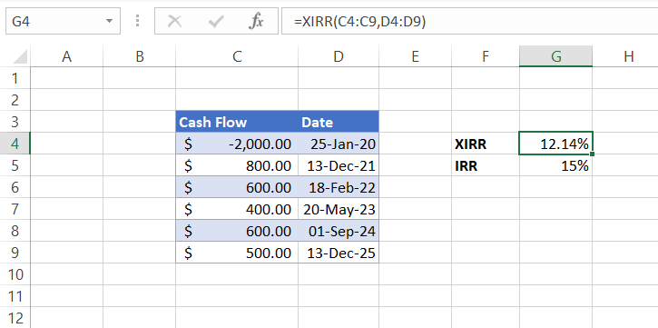
Assume that you invest $2,000 by purchasing a vending machine from eBay and expect to earn cash flows from it for the next five years. We can find the internal rate of return by using the following formula.
=XIRR(C4:C9, D4:D9)
Here, column D indicates the date of cash flows after eliminating the maintenance and inventory refill cost.
A business like this can have unequal timings of cash flows based on the owner’s preferences of withdrawing coins from the machine. When we compare IRR and XIRR for the same cash flows, we find a significant difference between the results given by both functions. This dissimilarity is created by unequal cash flows and can be reduced if the payments occur at regular intervals.
5. SUMIF and COUNTIF
The next advanced Excel formulas we will cover are SUMIF and COUNTIF. There is a slight difference between the two, which we will explain below. We will also show you an example of how to use both in Excel.
SUMIF Formula
The SUMIF formula is used to add numbers that meet specific criteria. The syntax for this formula is as follows:
=SUMIF(range, criteria, sum_range)
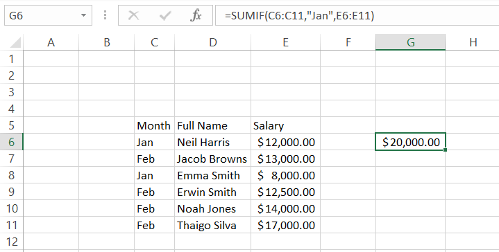
For example, if you need to find the salary given to the employees in January from the disoriented data below, you can use the above formula as shown below.
=SUMIF(C6:C11, ” Jan”, E6:E11)
In this example, our range is C6:C11, and our criteria is “Jan.” In this case, the sum_range would be E6:E11. This formula will return $20,000 because two salaries were paid in Jan.
COUNTIF Formula
The COUNTIF formula counts the number of cells that meet a specific criterion. The syntax for the formula is as follows:
=COUNTIF(range, criteria)
For example, assume that you are comparing loan amounts from two different spreadsheets during one of the reconciliation works for a mortgage lending firm. The data is as below:
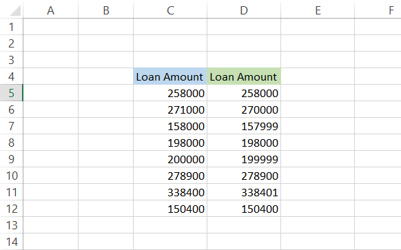
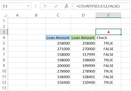
Now you must check whether the loan amounts from both spreadsheets reconcile. This can be done with a simple formula of =C5=D5. This will compare both values and give a TRUE result if values are the same and FALSE if values are different in column E. The final step is using the COUNTIF formula, which will summarize how many value comparisons return FALSE.
In cell E3, typing the following formula will give you a count of all the cells with FALSE as the value.
=COUNTIF(E5:E12, “FALSE”)
Since the significance of reconciliation is to highlight discrepancies in the data, such simple formulas make the task a lot easier.
4. PMT and IPMT
These two Excel formulas are used to calculate the payment on an installment loan. The PMT formula calculates the monthly payment, while the IPMT formula calculates the interest payment.
The difference between these two formulas is that the PMT formula calculates payments for a loan with constant interest rates. In contrast, the IPMT formula calculates payments for a loan with interest rates that change over time.
The syntax for PMT function is as follows.
=PMT(rate, nper, pv, [fv], [type])
where,
rate = interest rate for the loan
nper = number of payments for the loan
pv = present value of the loan
fv = future value of the loan. (Optional parameter)
type = indicates whether the payments are made in the beginning (type = 1) or end of the period (type = 0). (Optional parameter)
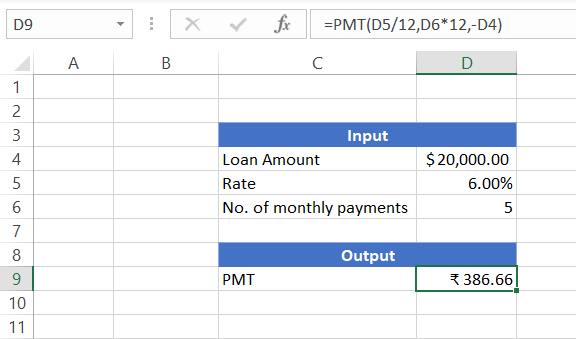
To use either of these formulas, you will need to input three pieces of information: Principle, Rate, and Number of Payments.
To find out how much your monthly payment would be on a $20,000 car at a 6% annual rate with a tenure of 5 years (60 monthly payments), you would enter the formula in a cell and get a result of $386.66.
=PMT(D5/12, D6, D4)
Since it’s an annual rate, we need to divide it by 12 for monthly installments.
Similarly, if we are paying the loan weekly, the same formula could be rewritten as shown below, and we will get $89.08 as the weekly payment on the loan.
=PMT(D5/52, D6*52, D4)
WSOs pro tip:
A negative sign in the formula for loan amount (PV) will give you a positive amount for the monthly payment amount.
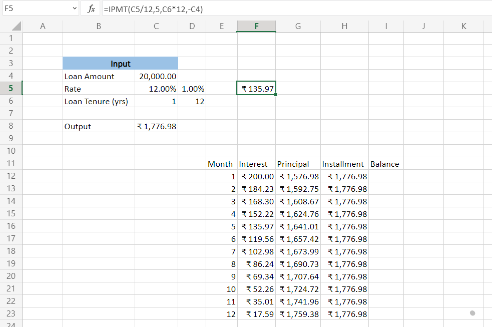
Suppose you have another loan of $20,000 for a car with a 12% rate that can be paid in a single year, i.e., in 12 monthly payments. What if you need to find how much interest you paid in the fifth month out of the total installment amount? You can use the IPMT function that will return you the interest paid in period ‘n.’ But first, you need to calculate PMT, which would be $1,776.98 in this case, using the below formula.
=PMT(D5, D6, -C4)
The syntax for IPMT function is:
=IPMT(rate, per, nper, pv, [fv], [type])
where,
rate = interest rate for the loan
per = number of payments over which interest needs to be calculated
nper = number of payments on the loan
pv = present value of the loan
fv = future value of the loan. It is an optional parameter.
type = indicates whether the payments are made at the beginning (type = 1) or the end of the period (type = 0). It is also an optional parameter.
Using the following formula will give $135.97 as the interest amount of the installment, while the rest is the principal amount ($1,776.98 - $135.97 = $1,641.01).
=IPMT(C5/12, 5, C6*12, -C4)
We have calculated the interest amount due for each month in the below table for your reference.
3. LEN and TRIM
LEN() and TRIM() are two Excel formulas that you’ll find yourself using more often than others. LEN(), also known as the length function, returns the length of a text argument by calculating the number of characters in the string. TRIM() is used to remove any leading or trailing spaces from a text argument except for a single space between words.
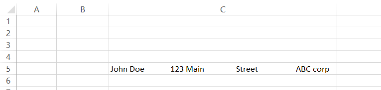
For example, assume that your data set has the following value in a cell.
“John Doe 123 Main Street ABC corp”
It has a lot of irregular spacing, making the data inconsistent with the other related fields and complicating the analysis.
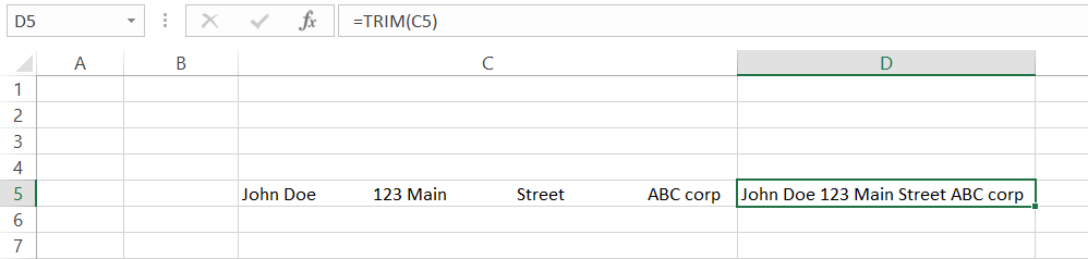
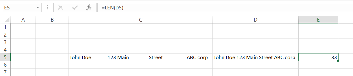
We can use the TRIM() function to remove the unnecessary spaces between text in cell C5. By using the simple formula TRIM(“C5”), you will get the result as “John Doe 123 Main Street ABC corp” and LEN(“D5”) will return 33.
WSOs pro tip:
The LEN() function will also count the unnecessary spaces as characters if you apply the formula in cell C4. To avoid this common error, we have used the LEN() function on the TRIM() result in cell D5.
In short, if you want to know how many characters are in a text string, use LEN, and if you need to know what is between two words with spaces, use TRIM.
2. CONCATENATE
The CONCATENATE function is a powerful function that will combine two strings of text, or two cells in a spreadsheet, into one.
This formula can be used when you have a list of people’s names and need to create a column with their full names. Simply type the names in separate cells and use this formula to combine them! For example, let’s consider the first and last names below and combine them into their full name.
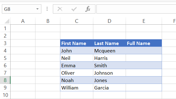
Below is the syntax for the CONCATENATE function.
=CONCATENATE(text1, [text2]...)
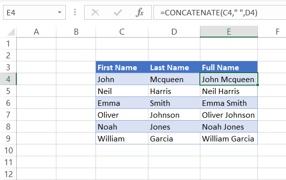
We will be using this formula with specific parameters given below to join the first and last name in column E.
=CONCATENATE(C4, “ ”, D4)
Do you notice we have used quotation marks with a space (“ ”) in between them in the formula? It is to produce the space between the two names without which we would get our result as “JohnMcqueen.”
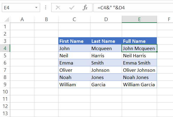
You can also use the &(ampersand) character to combine text from different cells to generate similar results. Below is the formula to concatenate strings using the ampersand character.
=C4&“ ”&D4
It is a matter of personal choice whether the analyst uses =CONCATENATE or the ampersand to join strings.
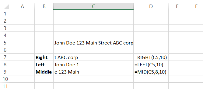
1. CELL, LEFT, MID, and RIGHT functions
The CELL function will provide you with information about a cell in Excel. The LEFT, MID, and RIGHT functions will extract characters from a text string. The LEFT function discards everything to the left of the first character. In contrast, the MID function takes everything between the beginning and the end, ignoring spaces between words, and the RIGHT function discards everything to the right of the last character.
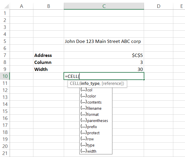
For example, assume that you have the value “John Doe 123 Main Street ABC corp.” in an unknown cell in Excel. To determine the cell address, we will use the below formula with “address” as the info type parameter to return the cell's address.
=CELL(“address”, C5)
Similarly, you can use different parameters to find information related to the cell.
Using LEFT, RIGHT, and MID() functions, we can extract characters out of one cell and into another cell. The num_chars is an optional parameter in the syntax for all three functions that determine the number of characters to be extracted from the selected text.
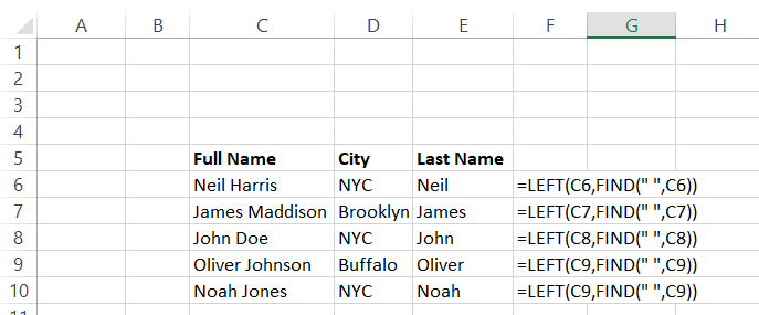
Using a combination including these three functions, you can extract data from an entire column or row in Excel without using many different formulas. For example, if you want to get every person’s first name in your spreadsheet, type the following in cell E6 and copy it down till E10 to separate the last names from the full names in column C.
=LEFT(C6, FIND(“ ”, C6))
Important things to remember
- A formula begins with the equal sign (=), without which any input function/formula will be represented as text in our spreadsheet.
- A space counts as a single character and must be considered while using functions such as MID, LEFT, RIGHT, and TRIM.
- Text values in formulas should be given inside quotation marks (“ ”). Else, the formulas won’t give you the correct value or show you an error.
Try Excel practice exercises with some of these formulas here.
More on Excel
To continue your journey towards becoming an Excel wizard, check out these additional helpful WSO resources.


or Want to Sign up with your social account?