VLOOKUP
It lets you look up and retrieve information stored in a table based on the value of an item in another cell


What Is The VLOOKUP Function In Excel?
The VLOOKUP function is an acronym for ‘Vertical Lookup’ and is one of the most indispensable tools in Excel. It lets you look up and retrieve information stored in a table based on the value of an item in another cell.

VLOOKUP is especially useful when you have data stored in two different tables related to each other. With this function, you can combine data from both tables into one easily readable format. Let’s take a closer look at how VLOOKUP works.
- VLOOKUP is an essential Excel function for looking up and retrieving information based on a value in another cell.
- The formula syntax for VLOOKUP is =VLOOKUP(lookup_value, table_array, column_index_num, [range_lookup]).
- Organize data with the lookup value on the left and the information to retrieve on the right for accurate VLOOKUP results.
- Be cautious of duplicates and consider creating unique identifiers to avoid incorrect results when using VLOOKUP.
- While VLOOKUP has advantages, such as simplicity and time-saving, it has limitations like static references and case-insensitivity, which should be taken into account during use.
Understanding VLOOKUP Function
VLOOKUP is a function that lets you look up data with the value of an item in another cell in a vertically organized table. To use VLOOKUP, input the item you are looking for in one of the columns in the table after which the function returns information from any row you like that corresponds to that item.
For example, we have the following employee data available for XYZ Inc.
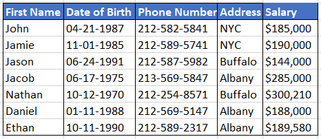
If we intend to determine Daniel’s salary, we can use the VLOOKUP function, enter “Daniel” into our formula, select the range, and VLOOKUP would return the salary as $188,000.
The VLOOKUP Formula
The VLOOKUP function is a simple formula that returns a value based on parameters in the formula.

The syntax for VLOOKUP is given by:
=VLOOKUP(lookup_value,table_array,column_index_num,[range_lookup])
where,
- lookup_value = The value to look for in the beginning of the table i.e first column value
- table_array = the table from which the value is to be retrieved
- column_index_num = this parameter intends to retrieve value from our expected column
- range_lookup = Optional parameter. TRUE gives an approximate match if exact match is not found, and FALSE gives an exact match or will return an error if an exact match is not found
The simpler version of the VLOOKUP syntax can be given as:
=VLOOKUP(the value that you are looking up, the range where you are looking for the value, the column number for the selected range in which the value exists, approximate match (TRUE) or exact match(FALSE))
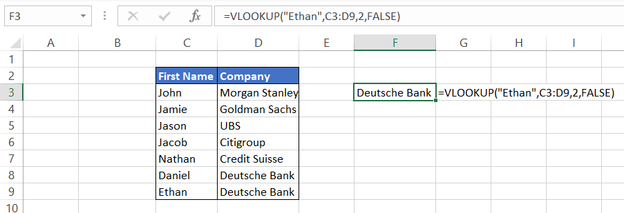
For example, we need to find the investment bank where “Ethan” works. Then, we can use the VLOOKUP function, which would return the value as “Deutsche Bank” as our result because it appears in column D at row 9 of the table.
how to use VLOOKUP in Excel
The VLOOKUP function is pretty straightforward to use. First, you’ll need to provide an example of the data you’re looking for and the table in which it’s stored.

The VLOOKUP function will then search the left-hand column in the table for a value that matches your search criteria and return a corresponding value from the same row.
Understanding how to use VLOOKUP can be a valuable skill. The correct use of this function can save time, reduce errors, and enhance efficiency.
STEP 1: Arrange your data from left to right
VLOOKUP can only find values to the right of the column being looked up, so if your lookup_value is at the end or in between the table, it will fail to retrieve the value and give you an error.
Instead, arrange the data so that the lookup_value is to the left, and all the corresponding information you need to retrieve is on the right side of the lookup_value to avoid getting the #N/A error.
STEP 2: Identify the lookup_value
lookup_value defines what the user is looking for. Excel is highly flexible and can look up names, numbers, and even dates. For example, in this case, our lookup_value list is in column B.
STEP 3: Define the table_array
The table_array argument guides VLOOKUP where to find the lookup_value and, if found, what value to return from the selected range or table.
You can choose the table_array from the same spreadsheet, a different spreadsheet, or even an entirely different workbook. In our example, the table_array is B5:E12.
STEP 4: Column_Index_Num
The column_index_num acts as a constraint and specifies the column from which we want to retrieve the value. These are defined by numbers rather than alphabets in our formula.
The VLOOKUP function cannot determine the column number by itself from which we want to retrieve the value, and hence the user needs to define the number in the formula.
Our table_array has four columns, and column_index_num can be either 1, 2, 3, or 4. (Using the column_index_num as 1 does not make sense and does not provide much value to the users.)
Note: You will receive a #VALUE! Error if the column_index_num is less than 1.
STEP 5: Choose between Exact and Approximate value
This is an optional yet the most crucial parameter of the VLOOKUP function. It commands Excel to find an exact or an approximate match for the lookup_value. The default value is always TRUE (1) if you don’t mention or skip the argument.
However, by using the FALSE (0), you can get an exact match for the data and avoid all the wrong results while looking for data.
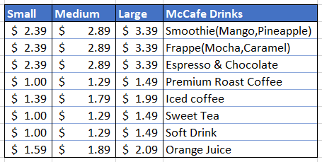
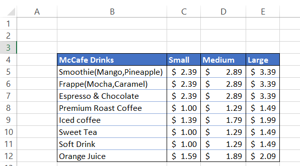
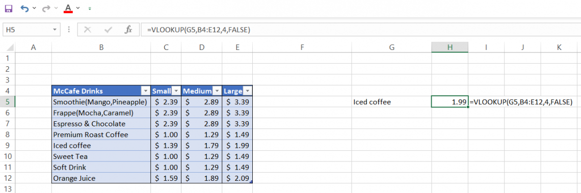
For example, let’s say we want to find the price of medium-sized Iced Coffee from the McDonald's menu. To do this, type the formula =VLOOKUP(G5, B4:E12, 3, FALSE)
In “McCafe Drinks,” we have a list of products with corresponding prices for small, medium, and large-sized drinks. We have referenced cell G5 to receive the price for different items on the menu dynamically.
In this case, the price of medium-sized Iced Coffee is $1.79. Similarly, if we want to find the price of large-sized Ice Coffee, we just need to change the column_index_num to the column from which we expect our value.
Here, we change our column_index_num from 3 to 4 by changing our formula to =VLOOKUP(G5, B4:E12, 3, FALSE).

When and why to use VLOOKUP
Whether you're trying to consolidate data from disparate sources, cross-reference records, or simply streamline your lookup tasks, VLOOKUP often presents itself as the optimal choice.

VLOOKUP is commonly used in two scenarios:
- When you’re looking for a value in a table and know in which column the value exists. For example, suppose if you have a list of customers with their contact information and know that customers’ age is given in column D. By specifying the column number, you can retrieve the age of the customers.
- To check whether a particular value exists in our data table. For example, if you are looking for the address of the employees in your database based on Full Name and the result gives you the #N/A error, it means that the address for the employee does not exist in your database.
VLOOKUP lets you specify the value you want to find or return in both cases. This is called the “lookup value.” You’ll also need to provide additional information about your lookup value, including what column it’s in and which table it’s in.
To do this, simply enter =VLOOKUP(lookup_value,table_array), where lookup_value is the value that links to your data set, and table_array is the name of the table that contains that data set.
VLOOKUP in financial modeling and financial analysis
When building financial models, you want to forecast what will happen in the future as accurately as possible. To do this, you need a lot of data from the past.

To forecast your future financial situation, you need to understand how the present conditions will affect the future. For example, if you are working on your income statement model predicting revenues in the upcoming years, how will it change your net income and earnings per share?
The VLOOKUP function is essential when creating these models because it lets you bring historical data into your model by linking it with current data.
Suppose you have made assumptions tables about the revenue growth driver in your financial model.
If your current annual revenue is $42,051 million and today’s date is December 15th, 2021, Excel pulls up an expected value for December 15th, 2022 of $45,205 million based on the revenue growth driver using the VLOOKUP function. You don’t have to calculate this yourself!

In the example above, we use the formula =O5*(1 + VLOOKUP($C$12, $C$5:$E$7, 3, FALSE)) to pull in the data from revenue growth driver assumptions in cells J5:N5.
By simply changing the value in cell C5 to either upside case or downside case, our financial model will reflect the revenue based on a 9% rate for upside case or a 6% rate for downside case.
Advantages of VLOOKUP
VLOOKUP brings to the table a set of advantages that can elevate any spreadsheet task to a new level of efficiency.

Some of the main advantages of this function are:
- Two modes of matching: Based on the selection of optional parameters TRUE or FALSE, the user can find either an approximate match or an exact match, respectively, based on the user preference.
- Easy to use: It is relatively easier to use once you get the hang of it as syntax components are straightforward.
- Saves time: By using VLOOKUP, the user can save time that is usually spent looking up the data manually or any other similar task.
Limitations of VLOOKUP
Understanding its limitations is crucial for maximizing its efficacy and ensuring the integrity of our data tasks.
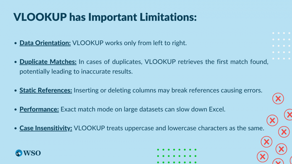
Some of the main limitations of the function to always keep in mind are:
- VLOOKUP always looks right: It means that your data must be oriented from left to right with your lookup_value at the extreme left. The function will not work if you intend to retrieve values to your left.
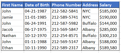
- Matches first value in case of duplicates: Suppose that you need to find the salary for ‘John’ from your employee database who lives in Buffalo. There is another John who lives in New York City.
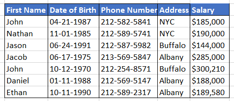
By using the first name as our lookup_value, enter the formula =VLOOKUP(H5,B4:F10,5,FALSE) in I5. This gives us the value of $185,000.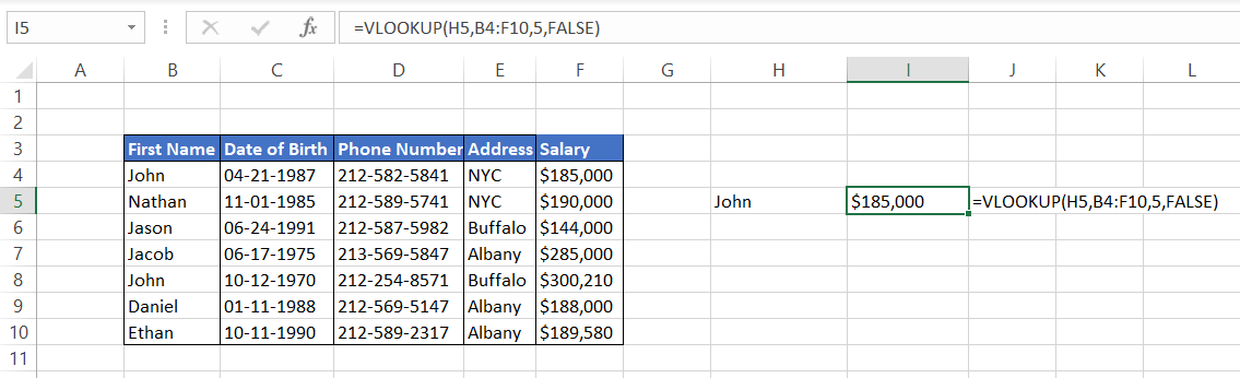 However, on closer inspection, we check that the results retrieved are actually wrong. Even after referencing the correct first name, the formula matches the result for the first value. Now, this is a small dataset. Do you think you can manually check spreadsheets containing hundreds and thousands of rows filled with data? (Don’t worry! We have got a bonus section on how to deal with duplicates later in this article)
 - Static references: If you insert or delete columns, you might get #REF! error as a result of references becoming invalid. In such cases, you need to edit the formula again to make valid references again.
- Slower calculations: When you use the ‘exact match mode’ on big data, it can cause Excel to slow down as it needs to iterate through every single cell of the table_array to find an exact match.
- It is not case-sensitive: When you want to retrieve a value, VLOOKUP treats ‘abc’ and ‘ABC’ as the same lookup_value, meaning it does not distinguish between them. This brings limitations in the usage of VLOOKUP on larger data sets.
Dealing with duplicates while using VLOOKUP
As an analyst, you will always come across datasets that consist of a significant number of duplicates. Since VLOOKUP will always give you the first value in case of duplicates, it is necessary to have some uniqueness in your lookup_value.
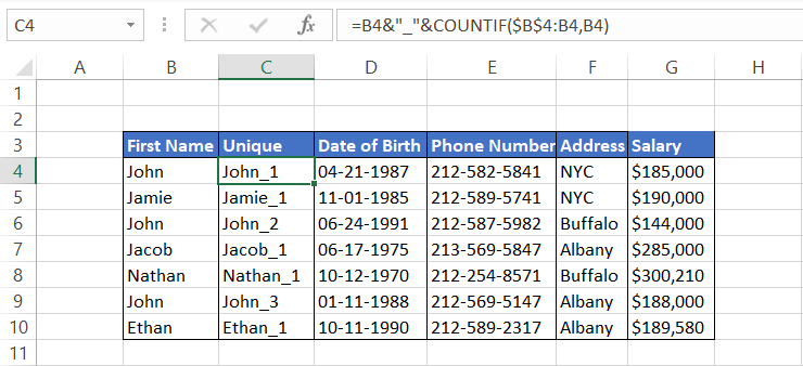
There you have it! That’s your solution to the duplicate values - unique identity. For example, suppose you have the below employee database consisting of three different ‘John.’
To retrieve the salary for the ‘John’ in the second-last position, we will be creating unique identities for First Name by using the formula =B4&“_”&COUNTIF($B$4:B4,B4) in cell C4 and dragging it down till the end of the table.
This is a combination of CONCATENATE and COUNTIF formula, which will add a column in your table as:
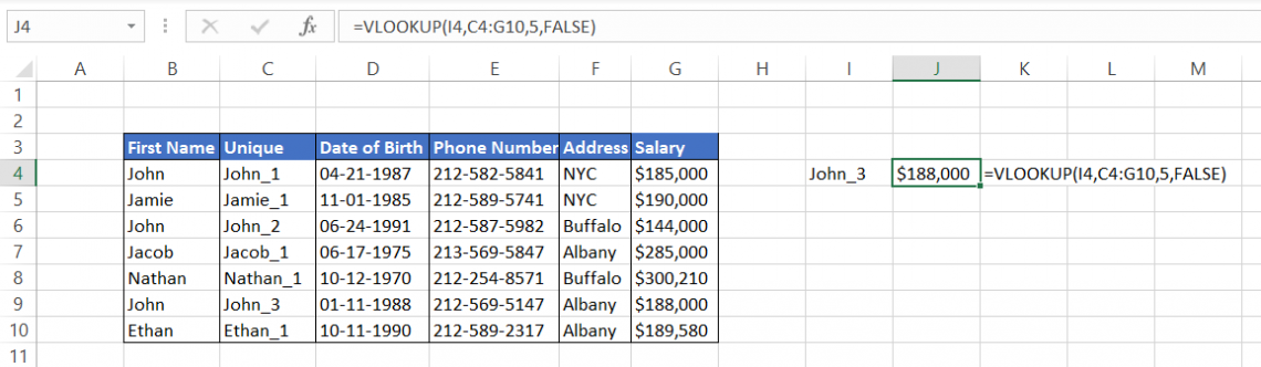
Now you can use the VLOOKUP function to find the salary for different John’s in your table. However, note that now our lookup_value changes from B4:B10 to C4:C10, and the table array becomes C4:G10. Including the B column in your formula will give you the #N/A error.
Things to remember about the VLOOKUP Function
VLOOKUP is a versatile function that lets you look up data based on the value of an item in another cell. You can use it to combine information from two tables or to search for something in one table based on some other criteria.
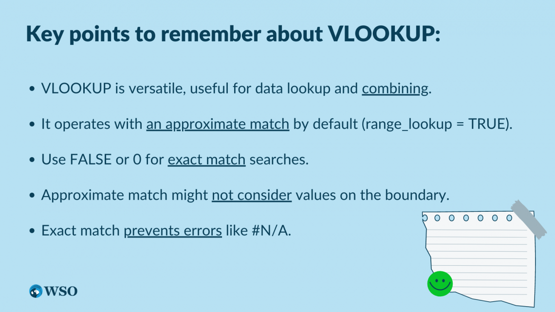
One of the most important things to remember about VLOOKUP is that it’s always looking for an approximate match, i.e., the range_lookup parameter is always set as TRUE. So, if you are looking for an exact match, the parameter must be set as FALSE or 0.
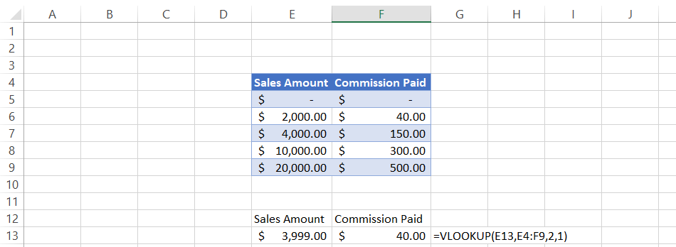
For example, if you were using VLOOKUP to find how much commission will be paid based on the sales made by the marketing team, then we will use the formula =VLOOKUP(E13,E4:F9,2,1) where the range_lookup is set as TRUE.
Even when the sales amount is $3,999, it does not add the commissions applicable on sales of $4,000. In this case, if we had used an exact match, we would have received the #N/A error.

Free Resources
To continue your journey towards becoming an Excel wizard, check out these additional helpful WSO resources.


or Want to Sign up with your social account?