Group in Excel
The best way to keep your spreadsheets organized

How to Group in Excel?
Ever worked on a cluttered spreadsheet, spending the whole night figuring out why your calculations are off, only to realize that some of the rows had been hidden and not updated? Some of us have.
And what about organizing data? What if your spreadsheets were more organized and readable? Wouldn’t it make you that much more efficient while making your work more presentable and understandable to a third party?
Maybe you want to train your juniors on working on the model you built or present the outputs of your model to your boss, who has no interest in looking at the raw data used to arrive at those outputs.
Well everyone has at some point in their career, wished that Excel had some functionality to organize data without having to keep track of where and what rows and columns have been hidden.
Worry not, as the people behind Excel know this too and have been generous to provide us with a powerful tool to organize data called the “Group” function, which is also known as the “Outline” function.
This comprehensive guide provides you with the knowledge you need to use this powerful function with ease and make it a part of your financial modeling toolkit.
The appeal of using spreadsheets such as Excel was due to their ability to make the results from analyzing data beautiful and meaningful.
As time passed, the most analytical industry, when it comes to number crunching and presenting to outsiders who may not like or understand technical lingo (i.e., finance), started heavily leveraging this powerful tool.
However, as with any flexible solution, it comes with its own problems that arise when the flexibility is misunderstood and misused.
Hide is one such tool that Excel provides, which is probably the most misused tool among new Excel users. There is a better tool that performs the same function but without its shortcomings called Group.
In the next section, we briefly talk about why hide should never be used, at least not in financial modeling, before going on to talk about the Group function.
- Utilize Excel's Group function to organize and summarize data effectively, avoiding the pitfalls of hiding rows or columns which can lead to errors and confusion.
- Grouping data in Excel allows for cleaner worksheets by collapsing sections of information when not in use, improving readability and presentation.
- Follow a structured approach to group rows in Excel: ensure labels are present, columns contain similar data, and there are no blank rows or columns within the range.
- Take advantage of Excel's Auto Outline feature or manually group rows by selecting them and using the Group function under the Data tab.
- Use shortcuts like "ALT + SHIFT + =" to reveal grouped data and "ALT + SHIFT + -" to hide it, enhancing efficiency and productivity in financial modeling tasks.
Excel Group Function
While building and working on modeling financial statements, there are a lot of rows and columns that, once filled and used to calculate an output, are better off “hidden” to have a cleaner worksheet with less clutter.
However, hiding rows or columns in Excel is considered bad practice, as it makes it very difficult for reviewers and future users to notice and account for the hidden cells.
This can and often will eventually lead to errors, especially when data from hidden cells are used as inputs to calculate output data in the non-hidden cells and are not updated.
For such situations, where we want to summarize the data and hide it when not in use, while providing an indicator of such hidden rows and columns, Excel gives us a handy tool called “Group.”
Group function allows us to summarize data into a maximum of 8 levels (it is uncommon to see more than 2 or 3 levels used; hence eight is more than enough). Furthermore, the grouped cells can be collapsed to hide the data until it is required, in which case, you would expand on it.
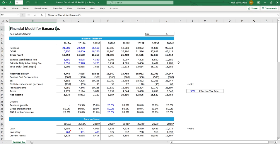
Source: A snapshot of a financial model from our Elite Modeling Package.
The Group function in Excel is among the most powerful functions that top analysts use to improve productivity while improving the presentation of their models. Financial models generally include complex and detailed information that makes reading and analyzing difficult.
There is no reason why you shouldn’t be using this tool to summarize your financial models and make the most of what Excel provides to come up on top.
Few of the most compelling reasons for summarizing data using this tool in your financial models are:
- To keep the data organized for future reference
- To avoid creating new sheets for every instance of similar data
- To hide or minimize data and calculations that are not needed by others
- To avoid the confusion that comes with using the default “hidden” function that Excel provides
- To expand and contract data as and when the need arises
How to Group Rows in Excel?
Below is a detailed explanation (changed for application in financial modeling) for creating an outline of rows in Excel as provided by Microsoft on their Excel guide.
- Make sure that:
- Each column of the data that you want to outline has a label in the first row, for example, EV/ EBITDA
- Each column you want to outline in the range contains similar data
- The range you want to outline has no blank rows or columns.
- If you want to add a subtotal row summarizing the data in the selected range, you can add it using two methods:
- Insert summary rows by using the Subtotal command
Use the Subtotal command from the outline ribbon, which inserts the SUBTOTAL function immediately below or above each group of rows and automatically creates the outline for you. Check out this guide provided by Microsoft for more information on the SUBTOTAL function. - Insert your own summary rows
If you are not comfortable using the SUBTOTAL function, you can insert a row for subtotal and manually enter the sum for each subgroup using the SUM function. For example, under the rows for Cost of Goods Sold (COGS) in the snapshot from earlier, use the SUM function to subtotal and arrive at the Gross Profit. The table later in this topic will show you another example of this.
- Insert summary rows by using the Subtotal command
- Now you have to outline the data you want to summarize. To do this, Excel provides you with a couple of options:
- Automatically outline data
- Select a cell in the range of cells you want to outline.
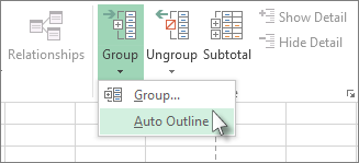
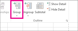
- Go to the Data tab, and in the Outline group, click the arrow under Group, and then click Auto Outline.
- Manually outline data
- To outline the data, select all the rows as well as any summary rows you have added to it.
- Go to the Data tab, and click Group in the Outline group. Then, in the Group dialog box, click Rows. Finally, confirm by clicking OK.
Tip: If you select entire rows instead of just cells, Excel groups automatically by row, without the Group dialog box appearing.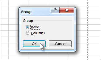
- Optionally, to outline inner, nested rows, select the rows adjacent to the ones that contain the summary row and proceed to step iv below.
- On the Data tab, in the Outline group, click Group.
 Then in the Group dialog box, click Rows, and then click OK. The outline symbols appear alongside the group.
Tip: If you select entire rows instead of just the cells, Excel automatically groups by row - the Group dialog box doesn’t even open. - Continue selecting and grouping inner rows until you have created all the levels you want in the outline.
- To ungroup rows, select them, and then on the Data tab, in the Outline group, click Ungroup.
- You can also ungroup sections of the outline without removing the entire level. First, hold down SHIFT while you click
 or
or  for the group, and then on the Data tab, in the Outline group, click Ungroup.
- To outline the data, select all the rows as well as any summary rows you have added to it.
- Automatically outline data
Summarized (Grouped) Data: How to Show or Hide?
Once you have created outlines from the important rows in your financial model, you would most likely want to hide or show the data as you please, depending on which part of the sheet you are working on.
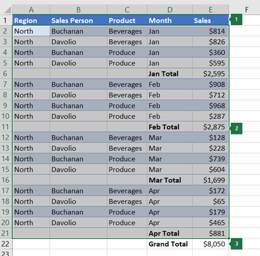
Your margin should now display outline symbols ‘+’, ‘-’, ‘1’, ‘2’, and so on. If you do not see these, go to File > Options > Advanced. Then, under Display options for this worksheet, enable Show outline symbols if an outline is applied. Finally, click OK to apply the change.
Clicking on the “+” button reveals hidden data used for the outline, while clicking on the “-” button hides the displayed outline. However, using the mouse is not something top analysts do as it makes them slow and less efficient.
To ensure that all WSO readers have a cutting edge in the industry, we provide and encourage you to use shortcuts for both functions. The shortcut to reveal the summarized data is “ALT + SHIFT + =” while the shortcut to hide the displayed outline data is “ALT + SHIFT + -”.
Since not all models are created alike or for the same audience, we recommend you go ahead and practice using these on your financial models to understand where and how to summarize data in a way that provides the best benefits to your specific use case.
Summarizing (Grouping) vs. Hiding data
There are many benefits to summarizing data in Excel. Think of the function “hide” as a subset of “group.” It provides a small implementation of the “group” but without all its benefits. Very often, hidden data is the cause of most errors while modifying or reusing spreadsheets.
While it is very annoying to deal with data you don’t need currently (yes, we know the frustration!), it is more annoying when your model throws out wrong outputs while presenting it to your seniors.
Not being able to find what’s going wrong in high-pressure situations doesn’t usually help with finding a solution. Hence, you should never use the “hide” function to hide data in any spreadsheet.
Instead, using the “group” function, which can be used easily with the shortcut we have provided, should be your priority. It may be tempting to use “hide” when the amount of data required to be hidden is small, but remember, the fewer cells you hide, the bigger the problem.
This is because finding one number missing in a sequence that runs to a few hundred is not easy and is the stuff of nightmares.
The video below from our Excel modeling course provides good instructions on how to use “group” like a pro and helps demonstrate the standards we help you achieve in your modeling journey.

More on Excel
To continue your journey towards becoming an Excel wizard, check out these additional helpful WSO resources.


or Want to Sign up with your social account?