Excel Drop Down List
A data validation tool that allows you to select an option from the given list of choices.


What Is Drop-Down List In Excel?
The dropdown list is a data validation tool that allows you to select an option from the given list of choices.
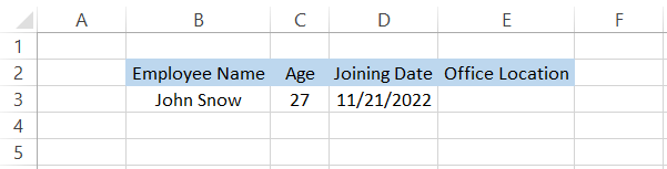
Suppose you are entering the employee information in the Excel database. Your office is present at two different locations - New York and Brooklyn.
When adding a new employee's information and assigning them an office, you can directly select the location from the dropdown list instead of manually typing the values.
The dropdown list can have a maximum of 32767 items, each of which can be selected by scrolling down the list.
Thus, instead of manually typing the values each time, the dropdown list makes it far easier to input values in the dataset.
Besides, it also acts as a validation tool to ensure that similar versions of the same values do not exist in the dataset. For example, if you need to input data in thousands of rows and one such value is 'Advise,' then there is a possibility you might add various versions of that particular value.
The variations can be 'Advice,' 'Advises,' 'Advices,' 'advice,' 'advise,' and so on. This can be prevented using the list, ensuring that only one value is consistently used in the entire dataset.
In the subsequent sections, we will see how to use the dropdown list and examples of combining it with functions to give you the best results in Excel.
- Dropdown lists are a valuable feature in Excel that streamlines data entry and ensures data accuracy by allowing users to select values from a predefined list of choices.
- Dropdown lists are created using the Data Validation tool, which can be accessed from the Data tab in Excel. This tool helps in setting restrictions on what can be entered into a cell, ensuring data integrity.
- Dropdown lists save time by eliminating the need for manual entry of repetitive values and prevent errors by enforcing consistent data input.
- Dropdown lists can be easily created by selecting the cell where the dropdown is needed, opening the Data Validation dialog box, specifying the list of values, and ensuring the "In-cell dropdown" option is checked.
Understanding Excel Drop-down List
As the name suggests, a dropdown list is a list of items open in the downward direction that allows you to select an option from the given list of choices.

The list can be created by accessing the data validation tool, which is present in Data > Data Validation in the Data Tools section.
A dropdown list plays two important roles for the Excel user:
- First, it avoids manual input of the same values repeatedly.
- Ensures data accuracy by preventing different versions of the same value, for example, advice, advices, advice, advice, etc., to avoid errors.
The list, if used wisely, can be a great tool for generating error-free reports of high quality.
In the next section, we will see how to create the dropdown list from absolute basics so you can modify the list you create.
How to create a Dropdown List in Excel
By reading the article so far, if you believe creating a dropdown list can be complicated, please let us prove you wrong.
You can create the list with just a few clicks, followed by referencing the values you need in the list.
Another prerequisite is selecting the cell in which you need the dropdown list.
Still confused?
It's all right. We will guide you step-by-step in this process and assure you that you will have mastered this awesome tool when you finish reading the article and get a couple of days of practice.
a. Selecting the cell and opening the Data Validation Tool
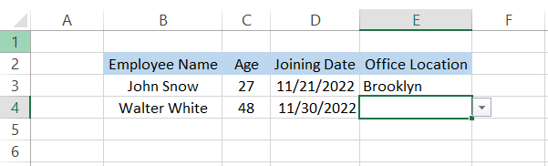
Suppose you have the data, as illustrated below:
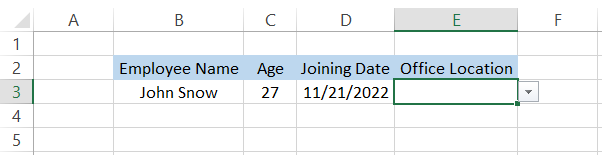
Like all other tools and functions in Excel, first, you need to select the cell you expect the list, which is the E3 cell.
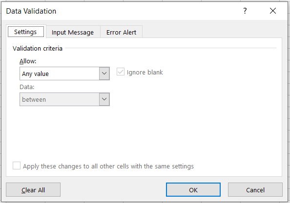
Click on Data > Data Validation, which opens the Data Validation dialog box:
Alternatively, you can press the keyboard shortcuts Alt + A + V + V, which would open the same dialog box.
b. Selecting the list and adding the values
Once the dialog box is open, you will find that the cell initially allows 'any value.' We will need to change this to a list and then input the values which should be present in the list.
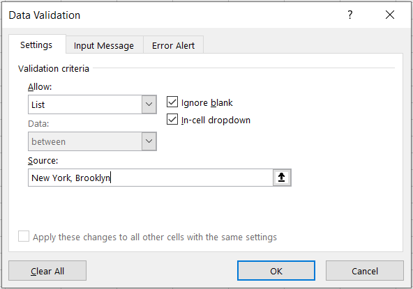
As shown above, now the values allowed are present in the list, whereas the source mentions that the values are New York and Brooklyn.
Here, we have hardcoded the values; however, you can also reference the cell directly.
The in-cell dropdown is an important checkbox that must remain ticked to get the list.
Finally, once you click on OK, you will find some changes in the selected cell.
c. Adding the value in the dataset.
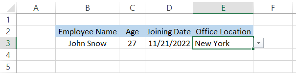
As the values are added to the list, the selected cell displays a button that can be clicked to assign a value to the cell.
If the employee is assigned to the New York office, you must click on the button and select 'New York'.
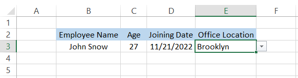
If the employee is transferred to an alternate location, 'Brooklyn' can be selected from the list.
Does this mean we cannot manually input values in cell E3? Well, the answer is yes and no.
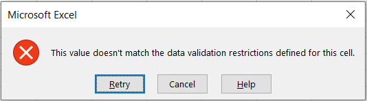
If we input value any other than 'New York' and 'Brooklyn,' we would get an error as illustrated below:

Even variations such as 'New York City' or 'Brooklyn City' won't work and will return the same error until you correct the value that matches data validation restrictions.
d. Copying the Data Validation rules to other cells
Following all the steps mentioned above can be tedious if we want the same validation rules in a different cell or a different spreadsheet.
Instead, what we can do is copy the cell with the dropdown list in cell E3 using the Ctrl + C key and then press the Ctrl + Alt + V key in another cell, which opens the dialog box:
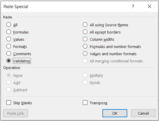
Here, we will select the radio button for 'Validation' and click on OK.
You will find that the cell now selected also consists of the same dropdown list with similar validation rules.
What Is Input Message?
When you open the Data Validation tool, you will find two additional tabs - Input Message and Error Alert.
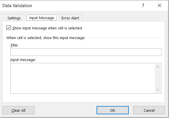
Input Message acts as a comment that lets you know what the different values you can expect in the list are.
For example, we will assign the title as 'Select Office,' and the description or the input message will be 'Office assigned can either by Brooklyn or New York.'
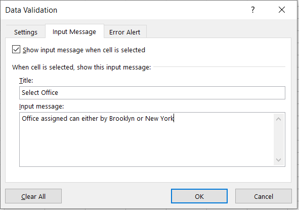
Another check box is ticked by default when you type in an Input message. If you untick the checkbox, you might not see the message when the cell is selected.
Once you click on OK if you select the cell with data validation rules, you will see something like
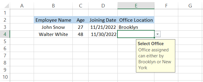
What title and message to assign entirely depends on you based on all the values in the dataset.
What Is Error Alert?
Finally, we have the tab for Error Alert. Previously, we saw that Excel gave us an Error whenever we tried to input a wrong value manually. This tab enables us to edit the contents of those error windows.
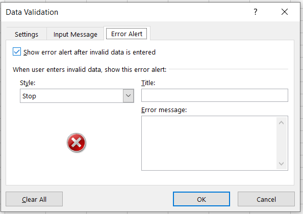
By default, when you input a wrong value, the error that you get looks as illustrated below:
Let's say we make some changes to the error alert window. First, the style is changed to 'warning,' and we have changed the 'Title' and the 'Error message' for the alert.
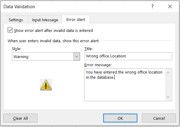
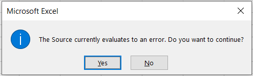
Click on Ok. Now try typing in values that do not exist in the dropdown list. You will get the error alert:
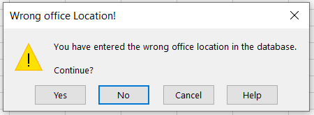
Here, you have four different options that you can choose from. You can either continue by clicking on 'Yes' or retry a different value by clicking on 'No.'
Well, that is all about the dropdown list in Excel. In the next section, we will see examples of combining the list and formulas to take data analysis to the next level.

Dropdown list along with formulas
One of the biggest advantages of using the dropdown list is its compatibility with all the formulas. You can directly reference the cell in the formula, and Excel will return the results accordingly.
Furthermore, you don't need to change the cell reference in the formula every time; you just need to select a different value from the list, and the formula automatically accommodates the changes.
This section will show examples of how you can use the dropdown list with the formulas.
a. COUNTIF function
The COUNTIF function counts the number of cells in Excel based on the condition that you input for a range of referenced cells.
If the condition is fulfilled, the cell is counted or skipped to evaluate the next cell.
For example, suppose you have the data as illustrated below:
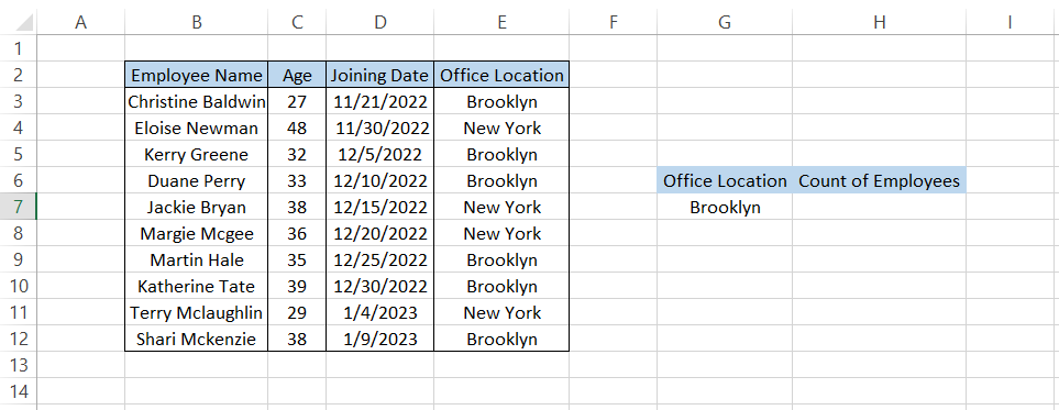
In cell G7, we have a dropdown list of the office locations for which we calculate the total count of employees.
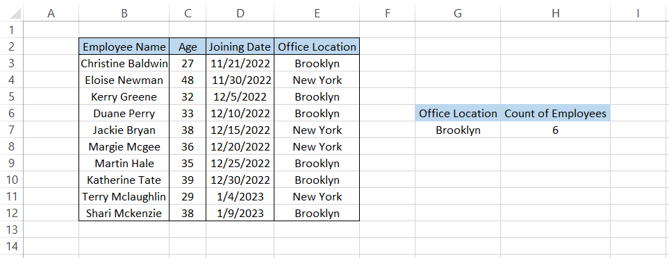
We will use the formula =COUNTIF(E3:E12, G7) in cell H7, which gives the number of employees in the 'Brooklyn' office 6.
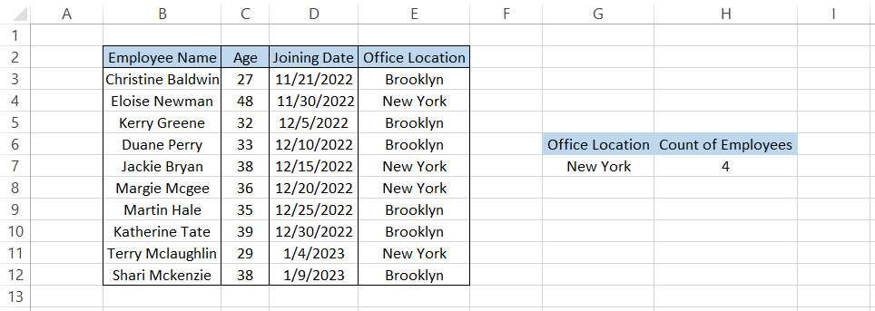
If we want to check the count of 'New York' employees, we don't need to input the formula again. All you need to do is select the value 'New York' from the list. This gives us the count of employees as 4.
b. VLOOKUP and SUM
VLOOKUP and SUM are two of the most well-known functions in Excel. If you are looking for a specific value in a vast ocean of data, then VLOOKUP is the right tool for you, whereas you know what the SUM function does.
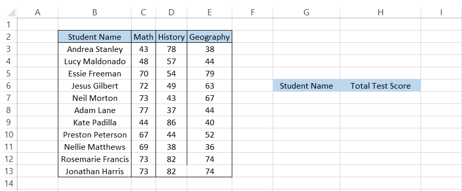
However, both can be combined with the dropdown list to make arithmetic calculations. For example, suppose you have the data as illustrated below:
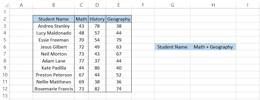
Firstly, we will create a list of all the students in cell B3:B12 using the Data Validation tool in cell G7.
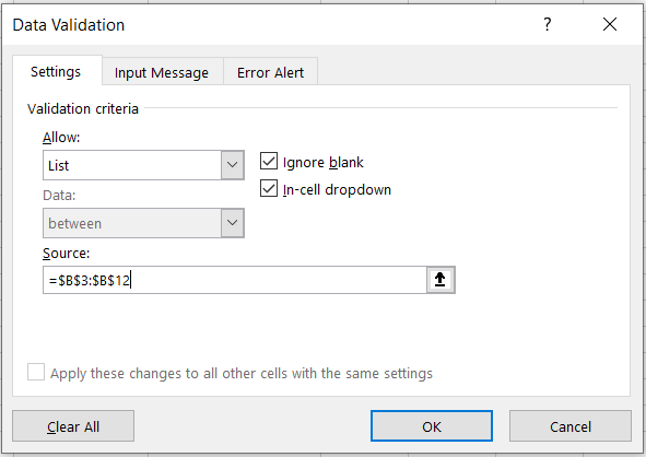
Click on Ok. Next, we will use the formula =SUM(VLOOKUP(G7, B2:E12,{2,4}, FALSE)) in cell H7 and press the Ctrl + Shift + Enter key to get the result.
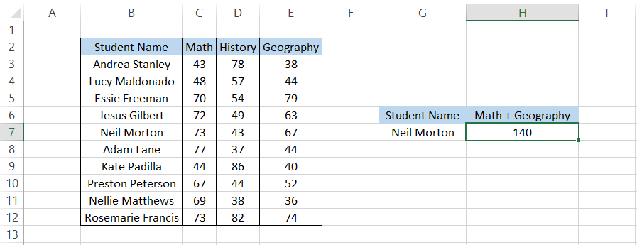
Unlike the traditional VLOOKUP, where we input just a single column_num argument, here you will find two since this is an array formula inside the curly brackets. This is because the numbers 2 and 4 inside the curly brackets correspond to Maths and Geography test scores.
If you change the student name from the list, the formula will automatically give you the sum of the Math and Geography test scores.
Instead of SUM, you can also use a different arithmetic function such as AVERAGE or PRODUCT.
Dependent dropdown list
Dependent dropdowns are those where the value from one list will generate an entirely separate list under that category. You can also think of it as branching of the data using the list.
An example could help us to understand better what dependent lists are. Suppose you have the data as illustrated below:
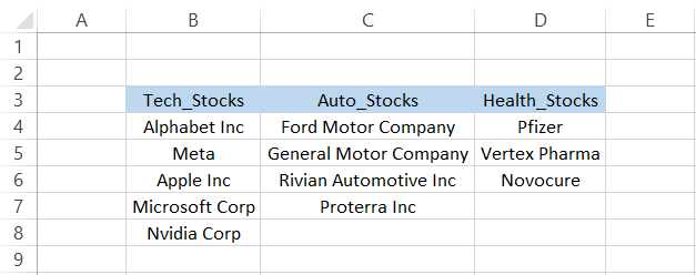
First, we will create a list using the headers in range B2:D2 in cell C9.
Next, we will select the entire data in range B2:D7 and click on Formulas > Create from Selection.
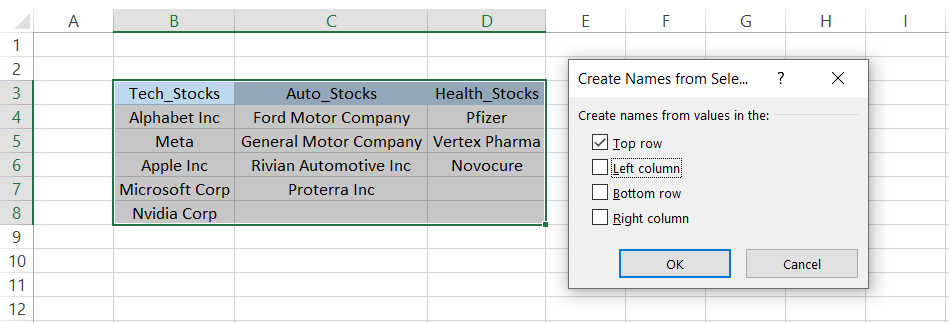
Next, we will create names from values based on 'Top row' and click on Ok.
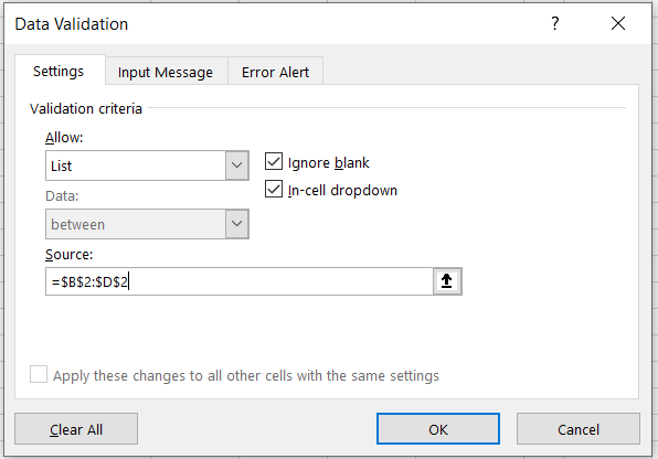
Finally, in cell D10, we will add another list where the formula in the source will be:

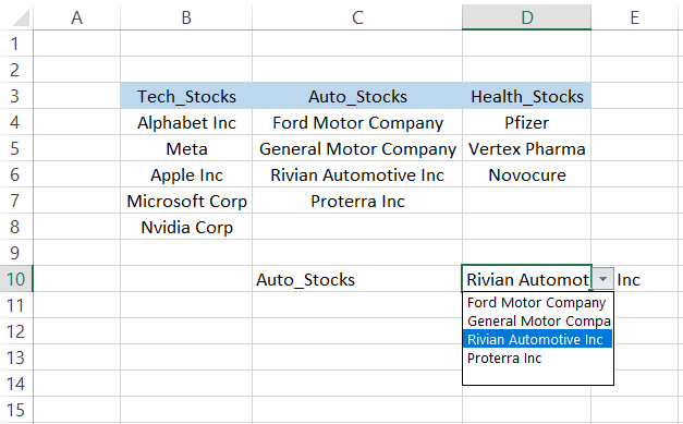
You will find that the headers are now linked to the underlying stocks in the dataset. For example, suppose you select Auto_Stocks in the list. In that case, all the auto stocks, such as Ford Motor, General Motors, Rivian Automotive Inc, and Proterra Inc, get suggested in a separate list in cell D10.
There is an extremely important point you need to remember. You must be careful, especially when using the 'Create from Selection' tool to create named ranges.
For example, we select the data in cell B3:D8 > Formulas > Create from Selection. Then, to check the named ranges, we click on Formulas > Name Manager to get:
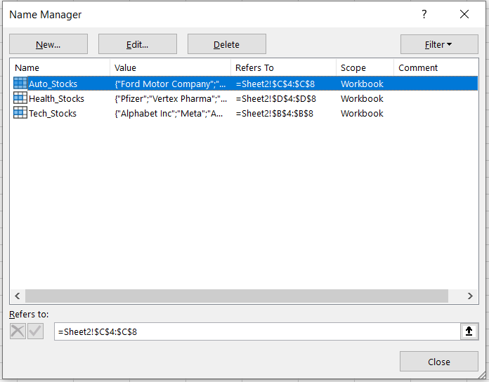
The ranges' names match the column headers in range B3:D3.
If the value in B3 was Tech Stocks(without the underscore), the dependent list would not have worked until you had added the underscore.
If you get an error, as illustrated below, just ensure that the headers from the dataset and the name ranges match each other, or else the list won't work.
This way, you can build up multiple lists that are all connected.
Dynamic Dropdowns
Finally, we want to shed some light on dynamic dropdown lists, which can be created in Excel with a few additional steps.
New data never stops generating, and preparing a static list can be quite annoying since we would have to update the list every single time.
In this case, we can prepare the dynamic dropdowns that automatically update the list if you add new values in Excel.
Suppose you have the student's test scores, as illustrated below:
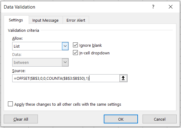
We will create the list from the Data Validation tool and input the formula =OFFSET($B$3,0,0, COUNTA($B$3:$B$50),1) in the source as
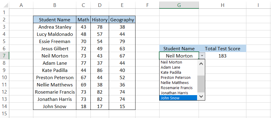
Once you click on Ok, you will find that the list has been created. Suppose that if new students are enrolled, and their data are added below the existing data, the formula will automatically update the list with the names.
For example, John Snow doesn't exist in our dataset. However, if we just type the value in B14 along with the test scores, we will see the name in the dropdown as:
The OFFSET function has five arguments:
- The first argument is our starting position of data which is cell B3.
- The second and third arguments are row and column, respectively. Since we do not want to resize our referenced range, we assign both values 0. As a result, the range remains B3.
- The next two arguments are height and width. Again, we use the COUNTA function for height and reference the range from B3:B50.
- Now, B50 is just an assumed number. You can input any cell number here in B50 but remember that the data won't automatically get added to the list beyond that cell. So, for example, new data won't be added to the list beyond the B50 cell in the range.
- The final argument is the width of the range. If we input a 0, then the formula will return an error. This means that the width of the data should be at least 1, which we have input in the formula to get a single column of data.
Also, we finally understand from John Snow's poor test scores why people always say, "he knows nothing."
Conclusion
Excel dropdown lists are a potent tool for increasing accuracy, speeding up data entry, and enhancing usability. By giving users a preset set of options, dropdown lists reduce the need for repetitive values to be manually entered.
This helps preserve data consistency across a spreadsheet.
Moreover, users may guarantee that data entering complies with predetermined criteria, lowering the chance of errors and enhancing data integrity, using features like data validation, input messages, and error alarms.
Excel formulas and dropdown lists work together seamlessly to enable effective data analysis and calculations depending on user-selected variables.
Features like dependent dropdown lists and dynamic dropdowns offer users additional flexibility and usefulness, allowing them to arrange and work with data more efficiently.

Free Resources
To continue learning and advancing your career, check out these additional helpful WSO resources:


or Want to Sign up with your social account?