AVERAGEIF Function

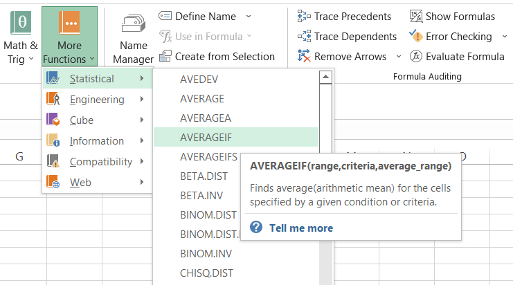
What is the AVERAGEIF Function?

The AVERAGEIF function calculates the average of values in a range that meets specific criteria. It combines two Excel functions: the IF and AVERAGE functions.

Using the IF function, each cell in a range is evaluated against the specified criteria, and the average of 'those' cells that meet the criteria is calculated.

The AVERAGEIF function can be used within a formula in a cell as it is a built-in worksheet function.

AVERAGEIF function Formula

The syntax for the AVERAGEIF function is:

=AVERAGEIF(range, criteria, [average_range])

where,

• range (required parameter): the range of cells to be checked for the criteria. It may include names, numbers, arrays, or numbers containing references
• criteria (required parameter): the condition that specifies which cells to average. It may include logical operators (such as "=", "<", ">"), text, numbers, or cell references
• average_range (optional parameter): the range of cells to be averaged. If provided, the AVERAGEIF function calculates the average based on this range; if omitted, it uses the same range specified in the 'range' parameter for averaging

How to use the AVERAGEIF Function in Excel?

Let’s look at different examples for the AVERAGEIF function that finds the mean of cells that meet our criterion.

Criteria based on text 

One of the easiest and simplest examples of the function is finding the average based on matching text. Let’s assume that the WSO fund buys stock for its portfolio. First, we must determine the average total buying amount for Tesla stock.

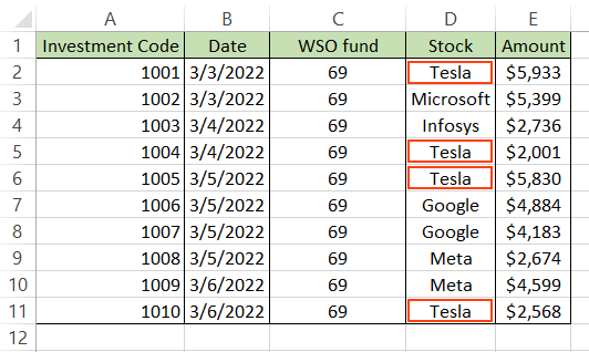
This can be achieved with the help of the formula =AVERAGEIF(D2:D11, “Tesla”, E2:E11), which gives us the result of $4,083. As we can see from the table, Tesla stock was bought in four instances, the sum of which equals $16,332.

However, since we are finding the average, the total amount gets divided by four to give us the final result of $4,083 ($16,332 / 4). 

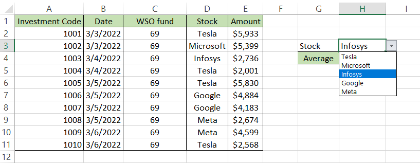
If you need to find the average amount for other stocks without changing the formula each time, you can use the data validation tool from the Data tab to let you have all the stock names in the drop-down menu.

You can change the stock from here, and Excel will find your average. The data validation tool can be accessed by using the keyboard shortcut Alt + A + V + V.

Criteria based on logic

The logical operators such as greater than (>), less than(<), equal to (=), greater than or equal to (>=), less than or equal to (<=), and not equal to (<>) can be used to calculate the average for a range of cells.

For example, assume that you need to find the average marks scored by students in the English subject.

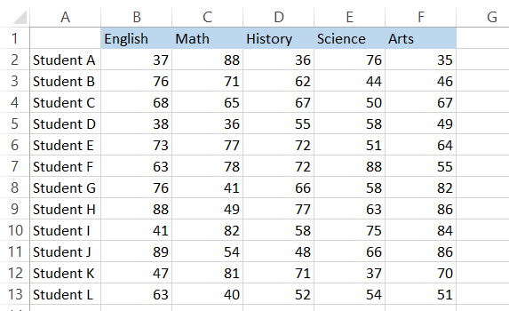
Here, you will use the formula =AVERAGEIF(B2:B13, ">55"), which results in 74.5 for the marks greater than 55 (condition) as illustrated below:
 

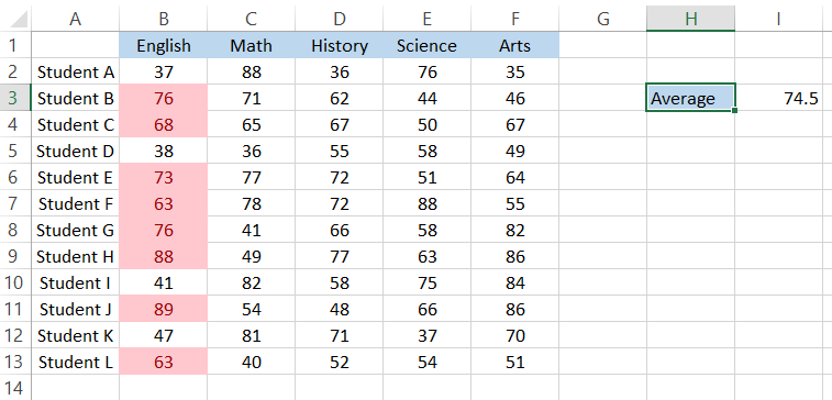
The formula only calculates the average for the highlighted cells and returns the result in cell I3. Notice that we ignored the third parameter average_range in our formula? Because we ignored the parameter, Excel assumed the range parameter for calculating the average value.

Criteria based on cell reference

You can find the average value based on hardcoded values in the formula and the cell references. For example, assume that 43 is the cutoff mark for English in cell I2. Then, you need to find the average for cells with scores higher than 43. 

To find this, you can use the formula AVERAGEIF(B2:B13, ">"&I2), which will give you the result as illustrated below:

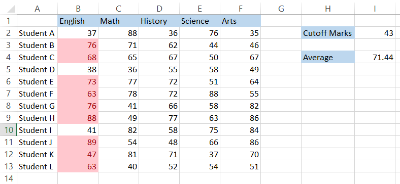
You can work with different scenarios for your dataset by concatenating the cell and the comparison operators. For example, if you get the result with recurring decimal numbers, you can use the ROUND function, so your formula becomes =ROUND(AVERAGEIF(B2:B13, ">"&I2), 2).

Not equal to the criteria

Not equal to criteria is best used when you want to exclude specific values from your result of average. For example, assume that you buy certain products from Amazon from one of their year-end sales. Your Amazon shopping cart looks as follows:

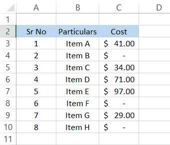
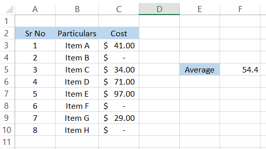
Since some items are free or on a 1 + 1 offer, their cost equals zero. Therefore, if you need to find the average price of the non-zero items, you can use the formula =AVERAGEIF(C3:C10, "<>0"), which will give you the result in cell F5 as:

AVERAGE of AVERAGEIF

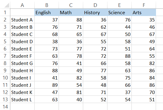
You can use a formula that works just like the AND function to find the AVERAGE of multiple AVERAGEIF functions. For example, suppose that you have the data for the marks scored by students in different subjects:
 

Let’s assume that you need to find the average marks of students who have scored more than 55 in English and Maths. To find this, you can use the formula =AVERAGE(AVERAGEIF(B2:B13, ">55"), AVERAGEIF(C2:C13, ">55")), which will give you the result of 75.96.

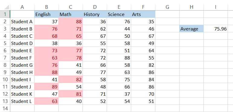
You can use up to 255 AVERAGEIF arguments inside the AVERAGE function to find the average of the AVERAGEIF.

AVERAGEIF for empty cells

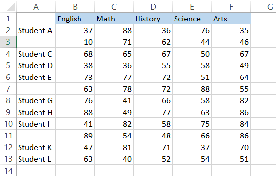
Sometimes, you might need to find the average for cells corresponding to empty cells. Assume that you have the data below where column A has missing students:

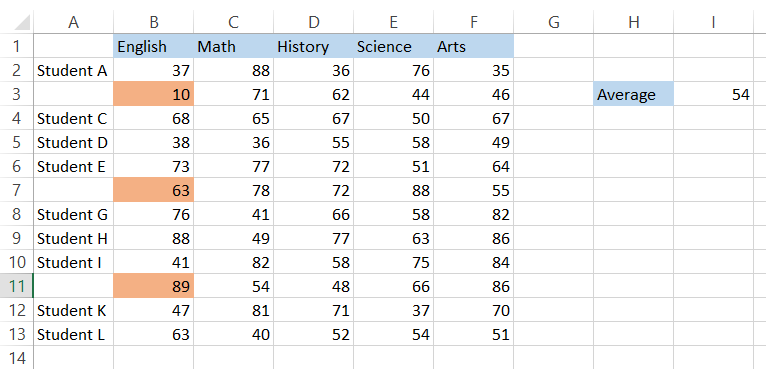
You can apply text-based criteria logic here to return the average number of cells corresponding to empty cells in column A.

The formula you will be using here is =AVERAGEIF(A2:A13, "", B2:B13), which calculates the average as (B3 + B7 + B11)/3 to give the result as 54, which is the average score of students whose names are missing.

AVERAGEIF with wildcards

Wildcards are \special characters that are used to return results by substituting them with other characters. The most common of wildcards used in Excel are:

• Asterisk (*) - can represent n number of characters before or after the wildcard. For example, ab* will return true for above, abduct, abandon, etc.
• Question mark (?) - can represent only one single character. If more than one question mark is used as a wildcard, you can return values based on multiple characters. For example, ?a will return true for values such as pan, van, fan, while ??t will return true for fat, cut, bet, etc.

Let’s look at an example to understand how to use these wildcards in real life. First, let’s assume that you want to find the average of expenses from your accounting journals that are illustrated below:

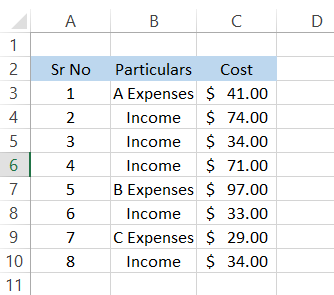
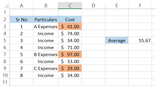
As you can see, all the expenses are represented by different names in the journal. Here, you can incorporate the use of wildcards by using the formula =AVERAGEIF(B3:B10, "*Expenses", C3:C10) to get the result of 55.67. 

Even if you write the formula as =AVERAGEIF(B3:B10, "*es", C3:C10), you will get the same result subject to the condition that no other word ends with “es” such as series, bikes, etc. 
 

Things to remember about the AVERAGEIF Function

Let's see what are the pointers that we need to keep in mind while using the function:

• If no value is assigned for the average_range parameter in the formula, it will be omitted. Instead, the formula returns the average for the range parameter based on the criteria
• Excel will return #DIV/0! Error if none of the cells meet the given criteria. For example, in the data below, we can see that none of the prices are greater than $25

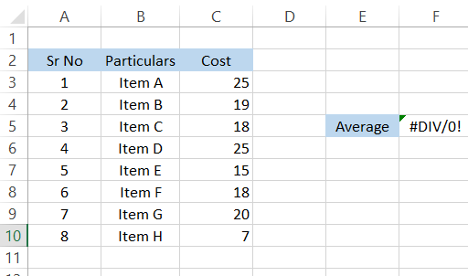
• If we use the formula =AVERAGEIF(C3:C10, ">40") to get the average individual cost higher than $40, we will get #DIV/0! Error since no values match our criteria
• Excel will return #DIV/0! Error if your range consists of text. For example, if you forget to include the average_range parameter for text-based criteria by mistake, it will assume that it needs to find the average based on the range parameter. As illustrated below, by using the formula =AVERAGEIF(C3:C10, "Item A"), we get the r#DIV/0 error

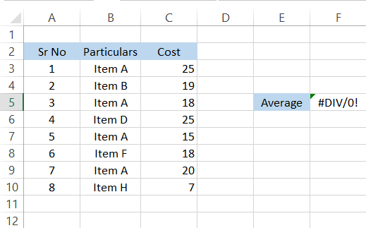
• If the criteria are text-based, you will need the average_range parameter in your formula

Free Resources

To continue learning and advancing your career, check out these additional helpful WSO resources:

• Countif Multiple Criteria
• Dynamic Dates, Sum, Average and Scenarios
• Excel Array Formulas
• Excel Formulas Cheat Sheet
• IFS Function