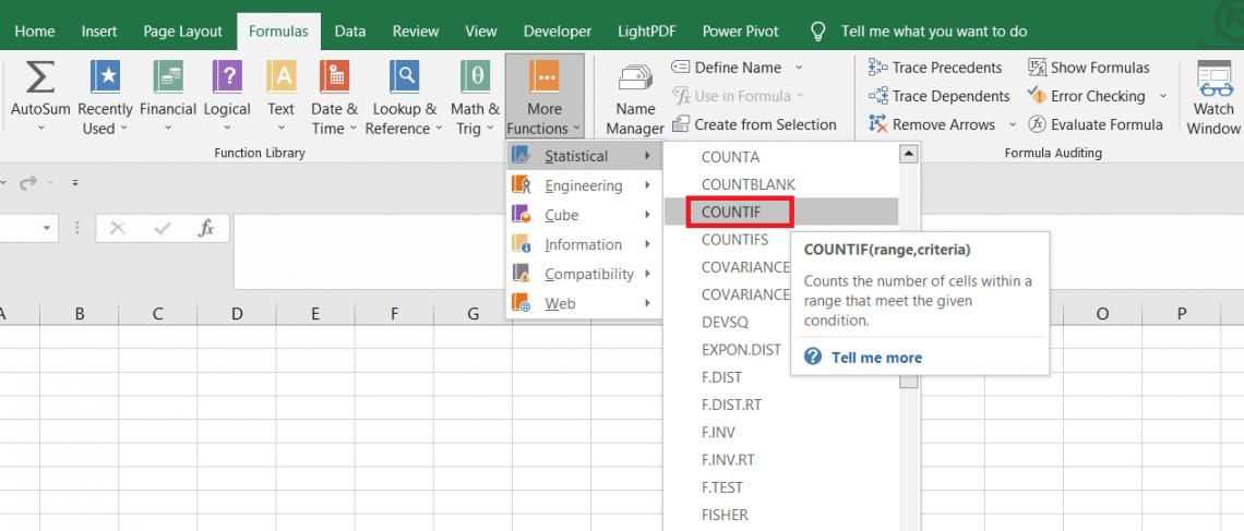
Countif Multiple Criteria
A function in Microsoft Excel that permits the user to count cells based on multiple criteria.


How to Countif Multiple Criteria?
The Countif Multiple Criteria is a function in Microsoft Excel that permits the user to count cells based on multiple criteria. There are generally two functions that let you count the number of cells based on predefined criteria - the COUNTIF and the COUNTIFS function.

The COUNTIF function accepts a single criterion to evaluate the cell count, while the COUNTIFS counts the cell based on multiple criteria.
As both of them perform identical tasks, they are often considered the same. However, we know that’s not the case.
As iterated earlier, the presence of the ‘n’ number of criteria forms the biggest difference between the functions and the eventual results that each returns to the user.
The comparison operators, which we will discuss in the subsequent sections of the article, can leverage the maximum potential of both functions.
Either of these functions also supports wildcard characters which can be used to make partial matches in Excel.
This article will guide you on how to use both functions and how you can use them to improve.
- The COUNTIFS is categorized as a statistical function that returns the count of cells based on multiple criteria.
- The COUNTIFS function accepts two arguments - range and the condition by which you want to count the cells. You can even add multiple criteria to the same range of cells.
- The function can accept 127 pairs of range/criteria combinations. However, only one pair is required for the function to work; the rest are optional.
- The comparison operators such as equal to(=), greater than(>), less than(<), greater than or equal to(>=), less than or equal to(>=), and not equal to(<>) can be used along with the COUNTIF function to improve the scope of financial analysis.
What is the COUNTIFS function?
Let’s focus on the important ones first. The COUNTIFS function is categorized as a statistical function that counts the number of cells specified by multiple criteria.
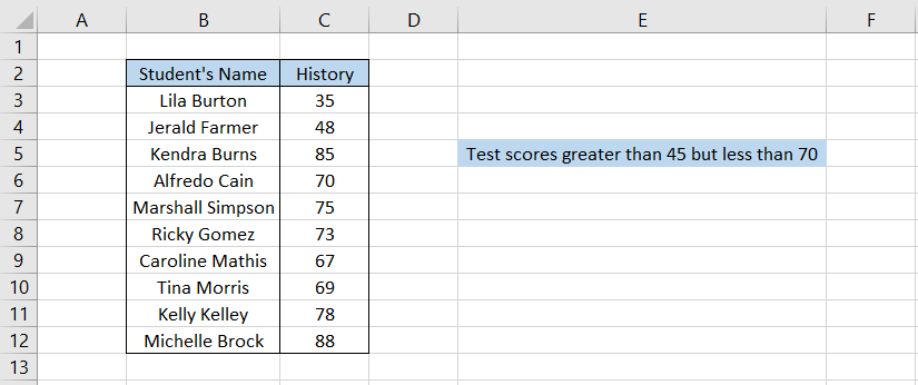
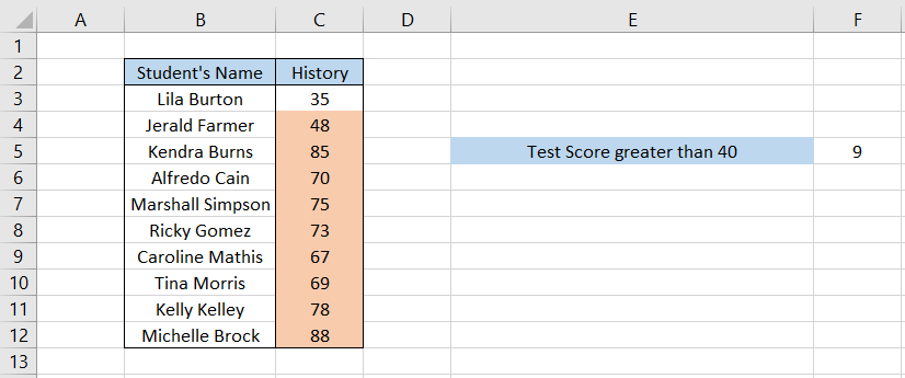
For example, suppose you have ten students' history test scores. Their lowest score is 35, while the highest test score is 88.
Let’s say the first criterion is to find all the students above the test score of 45. Additionally, the second criterion is to find the count of all tests below the test score of 70.
If we look at both criteria individually, the first will return the count of test scores above 45 up to a test score of 88, while the latter will return the count of all test scores between 35 to 70.
However, when you combine both criteria, the resultant count would be for test scores between 45 to 70.

The syntax for the COUNTIFS function is
=COUNTIFS(criteria_range1, criteria1,....)
where,
- criteria_range1: (required) the cell or range of cells that will be evaluated for the first criteria
- criteria1: (required) The first criterion
- criteria_range2: (optional) the cell or range of cells that will be evaluated for the second criteria
- criteria2: (optional) The second criterion
NOTE
The COUNTIFS function can accept up to 127 pairs of range/ criteria combinations to get the count of cells based on multiple criteria.
Comparison Operators
If you intend to make the best use of the COUNTIFS or the COUNTIF function, then there’s just one thing you need to include in the formula - comparison operators.

Comparison operators help compare two or more values present in different spreadsheet cells. For example, the greater than sign ‘>’ helps to check whether one number is greater than the other.
All these comparison operators are used to perform evaluations and are not limited to just the COUNTIF and COUNTIFS functions.
The different comparisons that you can use in Excel are:
| Operator | Description | Result |
|---|---|---|
| = | Checks if two numbers A & B are equal | (20 = 18) is FALSE |
| <> | Checks if two numbers A & B are not equal | (20 <> 18) is TRUE |
| > | Checks if number A is greater than number B | (20 > 18) is TRUE |
| < | Checks if number A is smaller than number B | (20 < 18) is FALSE |
| >= | Checks if number A is greater than or equal to number B | (20 >= 18) is TRUE |
| <= | Checks if number A is smaller than or equal to number B | (20 <= 18) is FALSE |
By using any of these comparison operators, you can easily increase the scope of your financial analysis and count the number of cells that meet the defined criteria.

Example for the COUNTIFS function
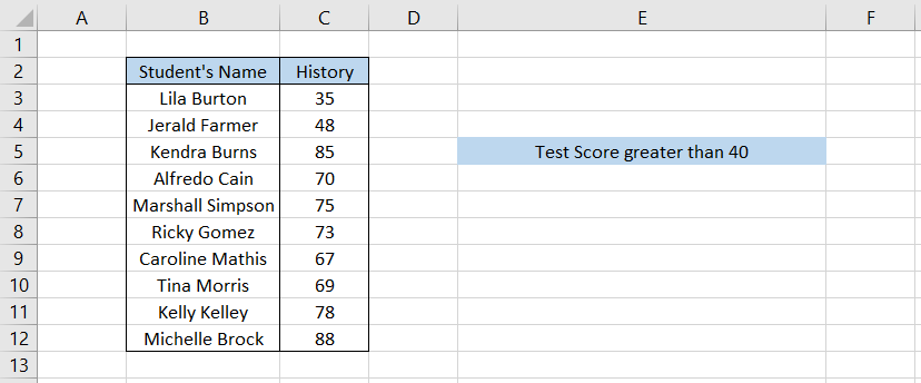
Let’s return to our example of test scores. Suppose the data looks as illustrated below:
We see that the highest test score in history is 88, while the lowest is 35. Also, let’s lay down the two criteria we will use to count the cells:
- The test score in History must be greater than 40.
- The test score in History must be less than 70.
When we combine both the conditions, the formula becomes =COUNTIFS(C3:C12,">40",C3:C12,"<70"), which gives the result as 3.
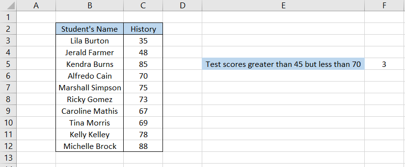
On closer inspection, we found that there were indeed three test scores that fell within the defined conditions.
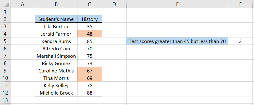
Since we used the ‘less than’ comparison operator and not the ‘less than or equal to,’ the test score of 70 is excluded from the cell count.
You can add even more conditions for the range C3:C12, and the function will find the cells that fit into those criteria.
Let’s see another example of the COUNTIF function.
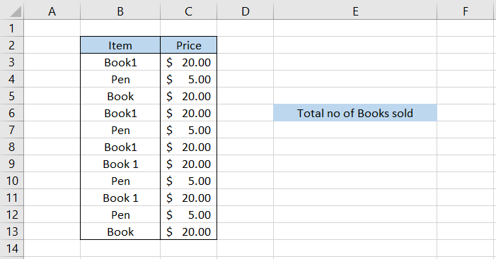
Suppose we have three different second-hand books sold at a store. If each book were bought new, the price would be $20. However, since the books are second-hand, they range between $5 and $20, depending on their condition.
The data looks as illustrated below:
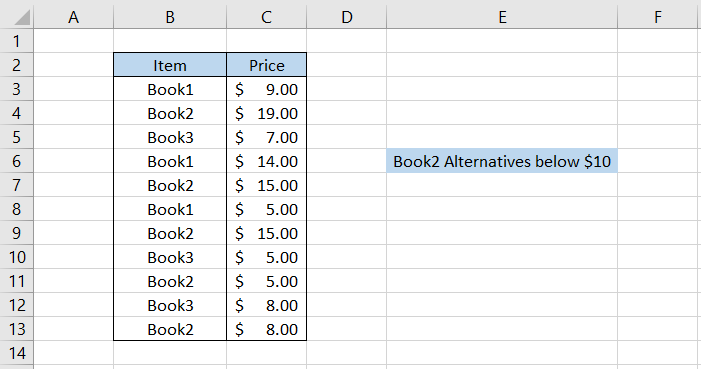
Suppose you want to buy book number 2, but you only have a budget of around $10. How many alternatives do you have to buy the cheapest one?
Here the two conditions are:
- Buying a Book2
- Price should be less than $10
The formula becomes =COUNTIFS(B3:B13,"Book2",C3:C13,"<10"), which gives the count as 2.
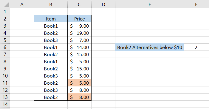
There are four Book2 listed; however, two are clearly out of our budget. The other two alternatives are $5 and $8.
Thus, the function could identify the text string condition of filtering the ‘Book2’ and then eventually return the count of those priced below $10.
What is the COUNTIF function?
COUNTIFS can test single or multiple criteria, so why do we still have a COUNTIF function?
The COUNTIF was originally the predecessor for the COUNTIFS function, which was introduced in 2007.
Before COUNTIFS, you could only input one criterion, and the COUNTIF function would give you the count based on the mentioned criterion.
Although the function has a new successor in the form of COUNTIFS, it is still operational and used by a significant population of users who aren’t aware of the capabilities of COUNTIFS.
The syntax for the COUNTIF function is:
=COUNTIF(range, criteria)
range - (required) the cell or the range of cells that will be evaluated for the given criterion
criteria - (required) the criterion to count the number of cells
Suppose we have the data as illustrated below:
We will use the formula =COUNTIF(C3:C12,">40") in cell F5 which gives the result as 9. Thus, there are a total of nine test scores that are greater than 40 in our dataset.
COUNTIF is a great alternative if you want to count the cells ‘only and only when’ you intend to use a single criterion.
If you have a single criterion right now but plan to add a couple more in the future, then always prefer to use the COUNTIFS function in such a scenario.
COUNTIFS and the Wildcard Characters
The beauty of both COUNTIF and COUNTIFS functions is that they allow the use of wildcard characters.

Wildcard characters are those that help to substitute other characters in their place. For example, assume you do not know the spelling of ‘Microsoft Inc.’ You do know that the first three letters are ‘Mic.’
Thus, using the wildcard character representing the rest of the characters, you can easily search the database and find all the matches that fit the criteria.
The different types of wildcards you can use in Excel are:
| Wildcard Character | Description | Example |
|---|---|---|
| Asterisk ( * ) | Can represent ‘n’ number of characters | he* will match all the words that begin with “he,” such as hello, hell, hey, etc. |
| Question Mark ( ? ) | Can represent only a single character | For example, ax?s can match words such as axes, axis, etc. It is for more specific partial match. |
| Tilde ( ~ ) | Nullifies the effect of a wildcard and returns them as a character | If the word is ‘Asterisk*, then we have to represent it as ‘Asterisk~*’ so that tilde nullifies the effect of asterisk. |
For example, suppose we have the data as illustrated below:
The store sells two products - books and pens. Each book and pen are of a single type and priced at $20 and $5, respectively.
A rookie accountant was recently hired, and he made the mistake of representing the same product under different names, but yeah, we are going to let it slide this time.
However, we want to know how many books were sold from the dataset. We can use the COUNTIFS function, but it would mean using many different criteria to accommodate the different text strings, which would take time.
Since we already know that each of the text strings begins with the letter ‘book,’ we can use the asterisk wildcard that will represent the rest of the characters that follow after them.
Then it can be the space followed by the number, just the number or nothing. The formula becomes =COUNTIFS(B3:B13,"Book*"), which gives the count of the books sold as 7.
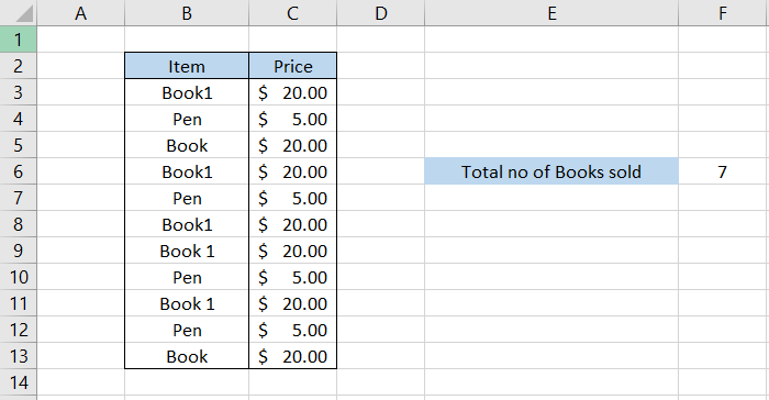
Thus, even though there were different varieties of text strings in the dataset, it could still identify every single one that met the criteria.
Let’s see another example for the question mark (?) wildcard character. Suppose we have the data as illustrated below:
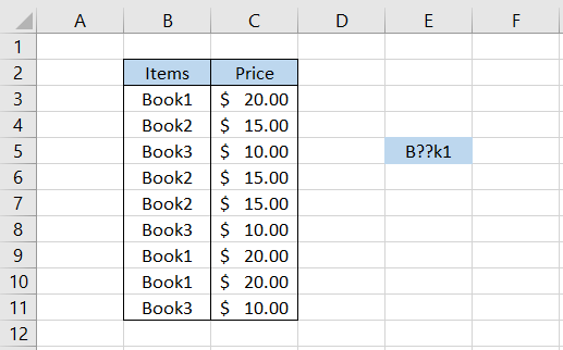
Let’s assume that we do not know the two characters from the item whose count we are looking for, as represented in cell E5.
To get the count using the wildcard, we will use the formula =COUNTIF(B3:B11,"B??k1"), which gives us the result as 3. On closer inspection, we find that there are indeed three line items that match exactly our wildcard + text string combination.
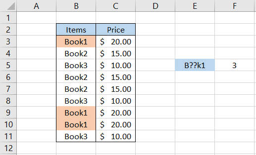
Thus, apart from the characters ‘B,’ ‘k,’ and ‘1,’ the formula would try to find all the characters that can replace the question. So, for example, if we had a text string as Brrk1, the formula would still count it as a match for our wildcard + text string combination.

Free Resources
To continue learning and advancing your career, check out these additional helpful WSO resources:


or Want to Sign up with your social account?