Index Match Formula
What is the Index Match Formula in Excel?


What is INDEX MATCH In Excel?
Index and Match are two of the most popular functions used in Excel. However, they can be combined together to form a tool that is more powerful than VLOOKUP and HLOOKUP in Excel.
You might wonder what is the need for the Index Match formula when the same results could be achieved with VLOOKUP or an HLOOKUP formula.
The reason it is preferred over VLOOKUP or HLOOKUP is that it allows the user to create two-way lookups, left lookups, case-sensitive lookups, and even lookups based on different criteria. There are many limitations to getting the desired result using the lookup formulas.
In this article, we will be illustrating why the combination of Index Match is superior to using the VLOOKUP as well as teaching you how to add this powerful tool to your modeling arsenal, something many people go on an Excel training course to learn.
To buy a copy of Excel or to learn more about this service, check it out here.
- INDEX MATCH is a powerful Excel formula, superior to VLOOKUP and HLOOKUP.
- It allows two-way, left, case-sensitive, and multi-criteria lookups.
- INDEX returns a value from an array based on specified row and column numbers.
- MATCH finds the position of a value in a range, supporting different match types.
- Combining INDEX and MATCH provides dynamic and flexible lookup capabilities.
How To Use The INDEX Formula
An Index function will return a value based on the row and column number specified from an array. It is given as:
=INDEX(array, row_num, [column_num])
where,
- array - range of cells that should return the required value. The subsequent row_num and column_num formulas are optional if the array consists of only a single row or column.
- row_num - the number of rows in an array from which the formula should return the value. The column_num is required if row_num is omitted from the formula.
- column_num - the number of columns in an array from which the formula should return the value. Since this is an optional field, the column_num is excluded if the required value is based on row_num.
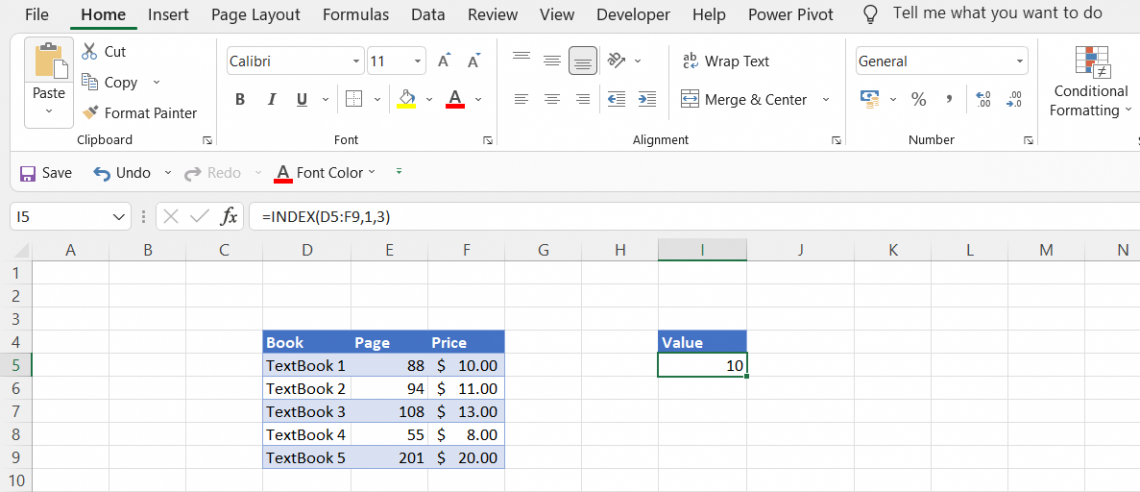
Illustrated below is an example of the Index function in action:
We use the Index function to return the value based on the intersection value of rows and columns. Here the entire range of cells is selected and the expected value is based on the row_num - 1 and column_num - 3, giving the final result of $10.00.
An Index function will also return the serial number of the given data if the formula is modified. Consider the example below:
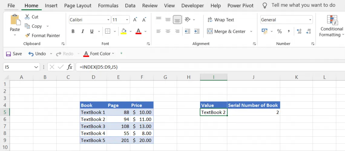
Here, the serial number (row_num) is hardcoded and used as the reference in the formula. When the range D5:D9 is selected using the formula INDEX along with the hardcoded serial number value, it will return the appropriate book as a result.
If the hardcoded value is changed to 2, it will automatically display the value ‘Textbook 2’. Remember that the considered array contains only a single column, so the column_num can be omitted in the function.
Another modification to the formula is using referenced values for both row_num and column_num to return the desired value from the array. In this example, the entire table is considered as an array, meaning it has three columns and five rows.
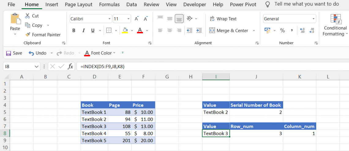
Here the selected array is D5:F9 for the INDEX function. The function will return the value based on the changes made in the row_num and column_num values i.e., if row_num is changed to 3 and column_num to 1, the value will be Textbook 3 which is the intersection of the third row and first column.
How To Use The MATCH Formula
The match function looks for a particular value in a range of cells and returns the relative position of that value in the referenced range of cells.
The match function is given as:
=MATCH(lookup_value, lookup_array, [match_type])
where,
- lookup_value - the expected value we are looking for. For example, when you are looking at the timing of the subway, you are using the train’s identification number to look up the value for the subway timings.
- lookup_array - the range of cells considered for the lookup_value
- match_type - this is an optional field that specifies how Excel correlates the lookup_value with the lookup_array. The match_type can assume three values 1, 0, -1 with 1 being the default value.
| match_type | Behavior |
|---|---|
| 1 | Requires "lookup_array" to be in ascending order, for example: -10,-5,0,5,10 to find the largest value which is less than or equal to "lookup_value" |
| 0 | "lookup_array" can be in any order for the match function to find the first value exactly equal to the "lookup_value". |
| -1 | Requires "lookup_array" to be in descending order, for example, 10,5,0,-5,-10 to find the smallest value which is greater than or equal to "lookup_value". |
Consider the examples below for the different match_type values:
For match_type value = 1 (less than), the lookup_array must be in the ascending order or it will display the #N/A error for the function. Here the lookup_value is 93 and the lookup_array is E5:E9.
By using the function =MATCH(93, Table1[Page], 1), the value obtained is 2. The lookup_value is less than the exact match of 94 from our lookup_range. Hence by using match_type 1, it gives the nearest number less than the exact match.
Confused what the solution will be if the lookup_value is 94? It's quite simple! The match function will give the position of lookup_value as 3 since it is an exact match. If your value is 100 and the nearest greater number is 108, you will obtain the match value of 94.

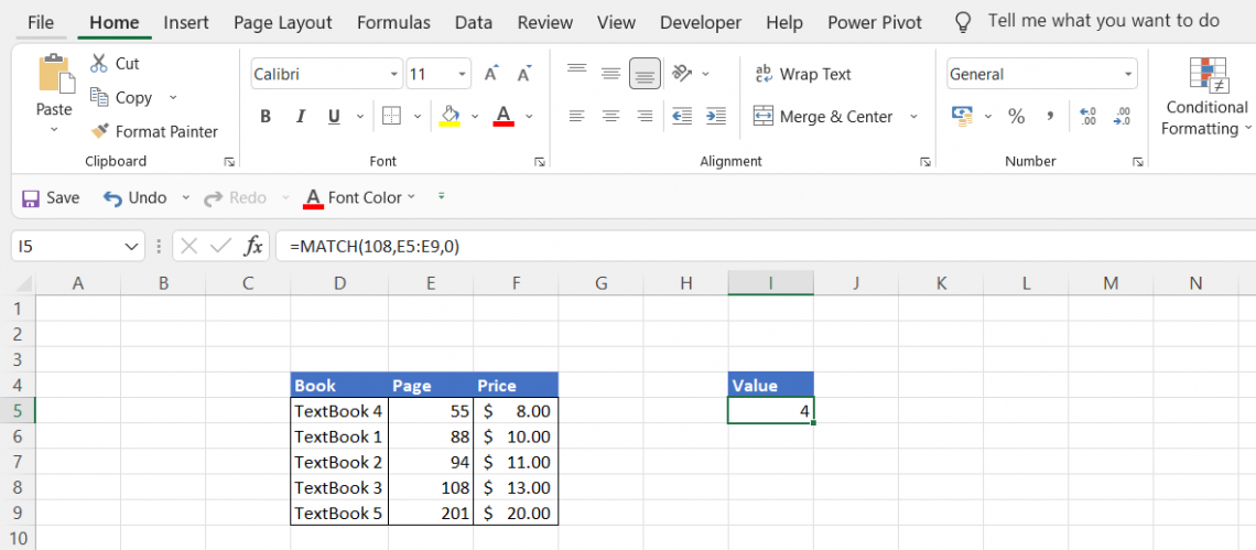
The lookup_array can be in any order if the match_type value is equal to 0 meaning that any lookup_value must return an exact value or else the function will display an #N/A error.
Assuming the similar values as above, by using the function =MATCH(93, Table1[Page], 1), the value obtained is #N/A as the lookup_value is not an exact match to any of the values in the lookup_array. If the value is changed to 108, the MATCH function will obtain result 4 as the position of value in the array.
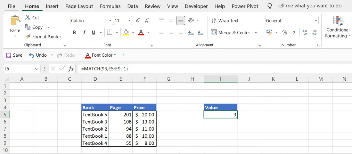
Contrary to the first behavior, the lookup_array must be in descending order for the match_type value -1 to return the smallest value greater than or equal to the lookup_value.
For lookup_value = 93 and lookup array E5:E9, the match function will give the value of 3 indicating that 94 in descending order comes closest to the lookup_value. If the lookup_value is equal to 56, the position value yielded by the MATCH function will be 4.
Combining INDEX MATCH formula
As we have now covered both the functions, we will now delve into how to combine them into a single powerful formula that returns the result.
The advantage of using this formula over the VLOOKUP function is that its lookup value can be in any column as opposed to values in the first column for the VLOOKUP function.
The interdependence of the two functions works in a way where:
- MATCH function will look for the values in the lookup_array and return its position based on the match_type criteria
- MATCH will relay the position of the value to the INDEX function
- The INDEX function finally translates this position into the result
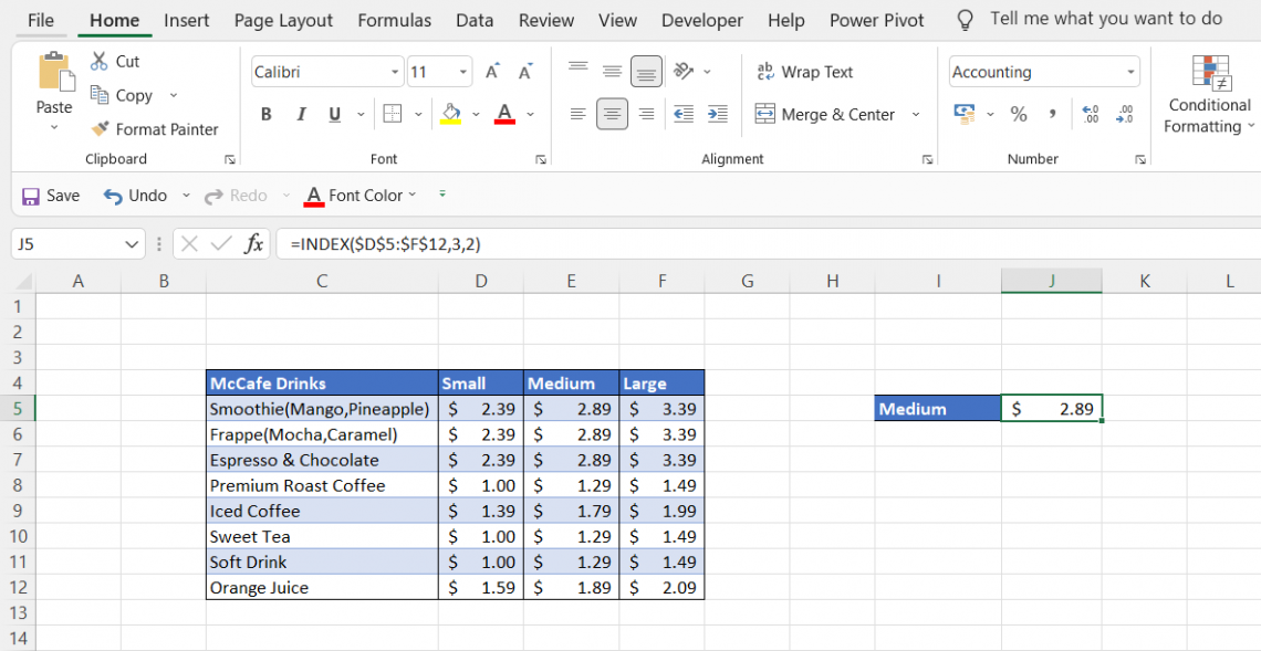
Consider the data below, a table showing a list of different McDonald’s drinks along with their price for different drink sizes: small, medium, and large.
Let's say we want to find the price of a medium-sized Espresso & Chocolate drink. Now if the data set is small like the following example we can just use the INDEX function as:
=INDEX($D$5:$F$12, 3, 2)
and it will return the result as $2.89.
However, it is always beneficial to use dynamic formulas in Excel as compared to hardcoded ones. You will need to change the row and column number for every unique search via the INDEX function. This can be overcome by incorporating the MATCH function.
Since we want to find the price of medium-sized drinks in this example, we will keep the column_num hardcoded in the INDEX function. By incorporating the MATCH function the formula becomes:
=INDEX($D$5:$F$12, MATCH(“Iced Coffee”, $C$5:$C$12, 0), 2)
and the result displayed will be $1.79.

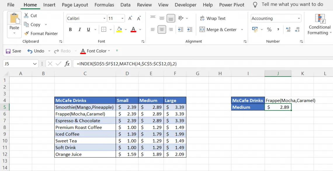
However, this still is not completely dynamic since you will need to update the hardcoded text in the MATCH function. To overcome this, simply place a referenced cell in the MATCH function which will spontaneously give the price of the drink.
The final formula used to find the price of a medium-sized drink is:
=INDEX($D$5:$F$12, MATCH(J4, $C$5:$C$12, 0), 2)
We know you might have a question in your mind. Why keep the column_num of INDEX function as hardcoded? Is there a way to make columns dynamic as well? Well, you have guessed the right answer.

Two-way lookup
We know that the MATCH function can be used horizontally as well as vertically. By utilizing two MATCH functions in a single formula - once to get the row position and the other to get column position, we can make the formula fully dynamic to find the price of the drinks of any size.
The formula we had earlier constructed was:
=INDEX($D$5:$F$12, MATCH(J4, $C$5:$C$12, 0), 2)
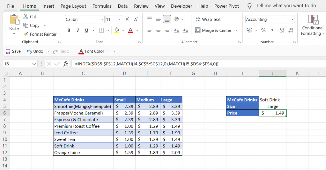
Substituting the value of column_num = 2 with MATCH(J5,D4:F4,0), we get:
=INDEX($D$5:$F$12, MATCH(J4, $C$5:$C$12, 0), MATCH(J5, $D$4:$F$4, 0))
Here we have already used the referenced cell =J5 in the second MATCH function as well to avoid hardcoded values of column names. When we press Enter, we get the price of $1.49 for a large soft drink. Similarly, by changing the values in cell =J4 and =J5, we can find the price for different-sized drinks.
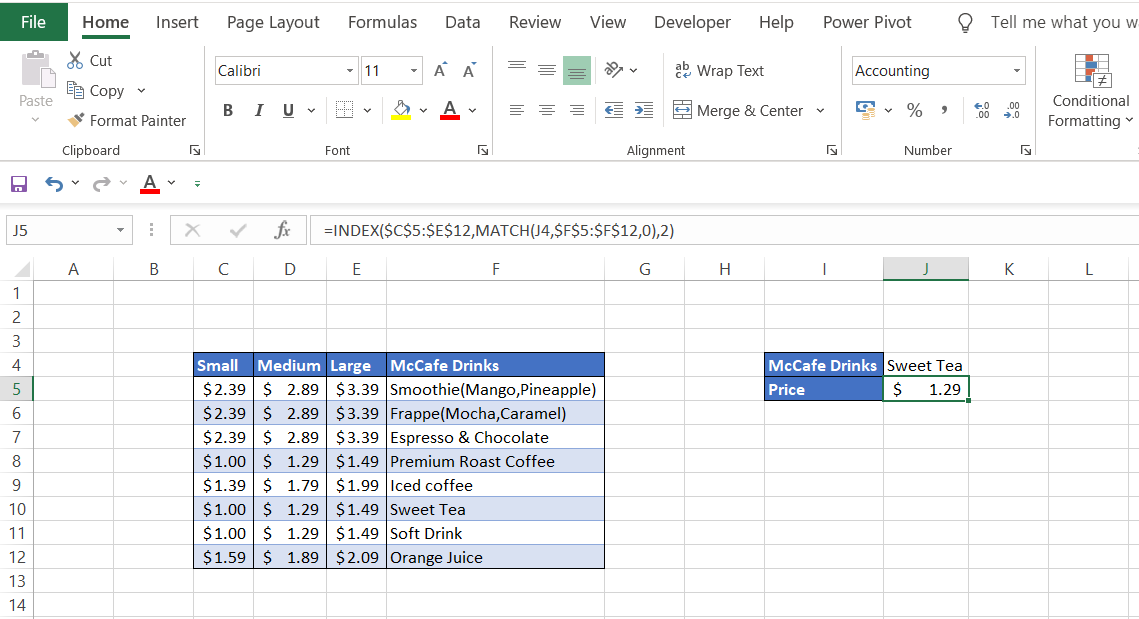
Left lookup
VLOOKUP is a powerful function, but one of its limitations is that it does not support finding values to the left of the lookup_value. A lot of times you will be required to find values to the left of the column, which is quite common while working on big data. This can be overcome with the help of the INDEX MATCH formula.
Consider the example below, where we have manipulated the data to look for values to the left. The column_number is constant (Medium) while the formula in the referenced cell J5 is:
=INDEX($C$5:$E$12, MATCH(J4, $F$5:$F$12, 0), 2)
This will give us the price of Medium-sized Sweet Tea in cell J5 as $1.29.
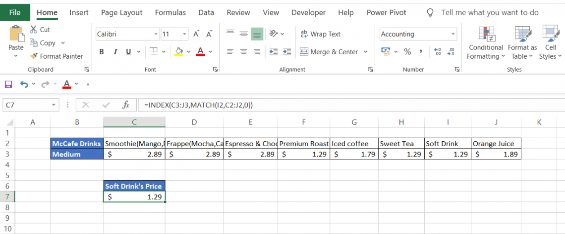
Horizontal lookup
What if you have similar data but instead of columns you have the data in rows format. Would you revert back to HLOOKUP to find the required value? Well, it is an option OR you could show your colleagues how awesome an Excel geek you are by using the combination of INDEX MATCH.
due to a change in the shape of the range, in this simplified example:
- The array for the INDEX function is C3:J3
- The lookup_array for the match function is C2:J2
By using the formula:
=INDEX(C3:J3, MATCH(E2, C2:J2, 0))
we get the price of the medium-sized Soft drink as $1.29.
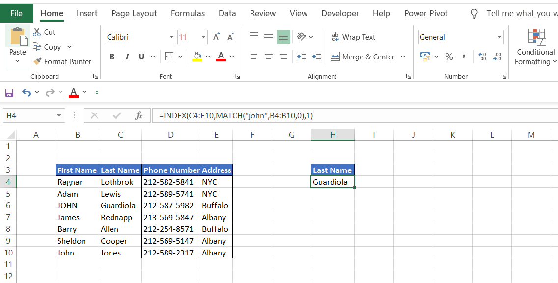
Case-sensitive lookup
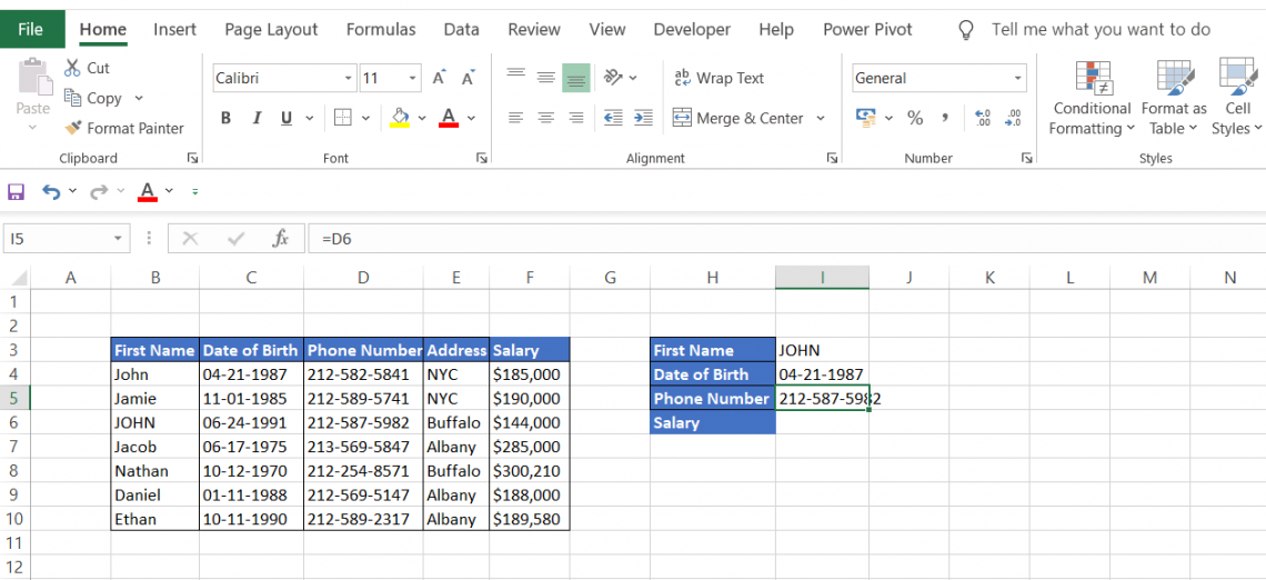
What if the data you are working on is case-sensitive? For example, your employee database could have two John’s where one is saved as JOHN while the other is just John.
Considering that you use VLOOKUP as well as the INDEX MATCH formula, you will receive employee information only for the higher ranking value in the data.
Assuming that ‘JOHN’ ranks higher than ‘John’ as depicted in the table below and you need to find the last name for ‘John’ but no matter whether you capitalize the lookup_value or write in lower text, the formula only gives the result for the one with last name Guardiola. So how do we overcome this problem?
The inclusion of the EXACT function in the INDEX MATCH formula helps to perform case-sensitive lookups in the data. The formula:
=INDEX($C$4:$C$10, MATCH(TRUE, EXACT(I3, $B$4:$B$10), 0))
gives the last name Jones for the other ‘John’ in the data. How does the EXACT function make the difference here? The EXACT function is given by the syntax:
=EXACT(text1, text2)
where text1 and text2 are the two strings that are to be compared.
Here we have assigned the First Name as text1 while the array in which we expect to find the First Name is assigned as text2. The formula is:
=EXACT(I3, $B$4:$B$10)
After going through all the values in the array, it will return TRUE only for ‘John’ while all the other values will turn FALSE. The output of the EXACT function for array B4:B10 will be {FALSE; FALSE; FALSE; FALSE; FALSE; FALSE; TRUE}.
Since we need the TRUE value, this is fulfilled by using the MATCH formula. The revised formula below pinpoints the required first name ‘John’.
=MATCH(TRUE, EXACT(I3,$B$4:$B$10)
The final step is to find the last name using the INDEX in the formula.
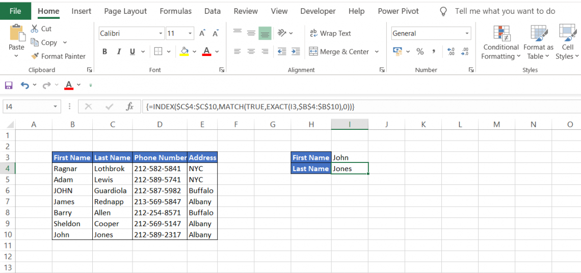
WSO's Note: Array Formula
Since this is an array formula, you must press Ctrl + Shift + Enter in the cell to display the result, or Excel will give an #N/A error (except in Excel 365).
Multiple criteria lookup
Many times while working on an extremely large database, a situation may arise where you don't have a unique identifier while looking for something. A lookup formula with several conditions is the only solution for such a problem.
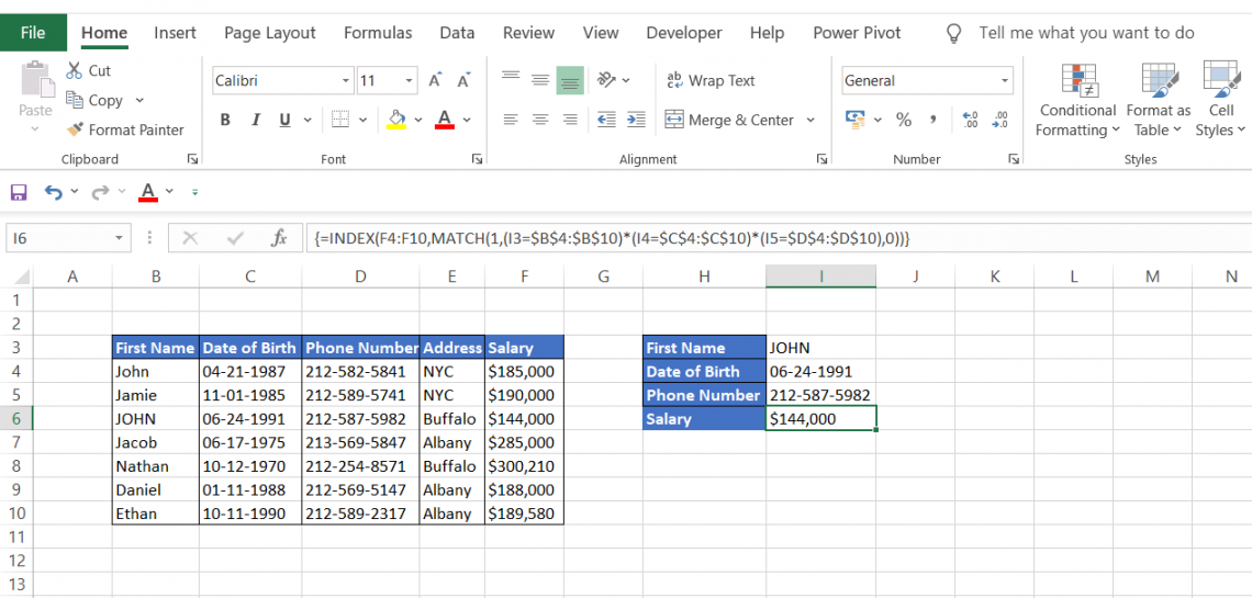
Consider an example where you are looking for the salaries of the employees working in your private equity firm. Let's assume you need to find the salary for capitalized ‘JOHN’ in your database.
You can set up two different unique criteria to obtain the salary for JOHN. This can be fulfilled by incorporating the date of birth and phone number array in the formula. Since ‘Address’ is not unique for the employees in the database, it will not be helpful as lookup criteria.
The final formula to look for the salary will be:
=INDEX(F4:F10, MATCH(1, (I3=$B$4:$B$10)*(I4=$C$4:$C$10)*(I5=$D$4:$D$10), 0))
Let's break up the formula to understand it better. Here are the three conditions:
- (I3=$B$4:$B$10)
- (I4=$C$4:$C$10)
- (I5=$D$4:$D$10)
These three conditions create boolean logic and give the result in the form of TRUE or FALSE for the lookup_value. For example, for the first condition (first name), the array will give the result of {FALSE, FALSE, TRUE, FALSE, FALSE, FALSE, FALSE}.
This can also be interpreted in 1’s and 0’s where 1 equals TRUE and 0 equals FALSE.
Thus, the three criteria can also be represented as:
(0,0,1,0,0,0,0)*(0,0,1,0,0,0,0)*(0,0,1,0,0,0,0)
The multiplication of these three arrays will give a final result of (0,0,1,0,0,0,0) which is used in the MATCH function will give the position of the lookup_value i.e. the third row in this case.
After this INDEX function works on this position derived using MATCH function and returns the salary of JOHN as $144,000.
Note
Since this is an array formula, you must press Ctrl + Shift + Enter in the cell to display the result, or Excel will give an #N/A error (except in Excel 365).
Partial match lookup using Wildcard characters
Sometimes your data might not be an exact match, making it difficult to use the lookup formula. At such times, you can find the required values by using an asterisk (*) in the formula which is a wildcard character to avoid getting the #N/A error in Excel.
For example, below are some of the listed companies on the stock exchange along with their stock price.
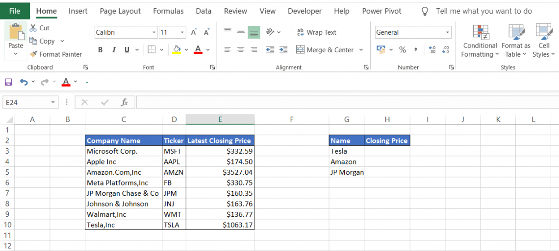
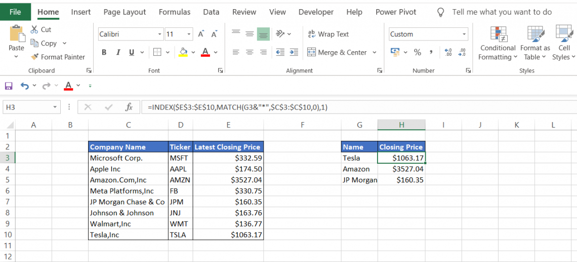
Notice that the lookup_value are not an exact match to the values in column C. However, a minor change in the formula can help to find the required closing prices of the stock. The formula that can be used is:
=INDEX($E$3:$E$10, MATCH(G3&"*", $C$3:$C$10, 0), 1)
The part of the formula G3&”*” represents that the text string after the cell value ‘Tesla’ can have ‘n’ number of characters forming the base of this unique lookup formula. Thus it gives the result as cell C10 i.e. the position of Tesla, Inc.
Once the position of the company name is determined, the INDEX function matches it to the stock price to give the value of $1,063.17.
Closest match lookup
Suppose that you are on a road trip and need to take a quick detour to one of the shortlisted locations on the map. Your car needs a refill as well which can be done only when you reach your destination. You decide that whichever place is closest to 150 miles will be your target destination.
How would you decide where to head next? Comparing our hypothetical example with large databases, at such times combining functions such as MIN and ABS can help to accomplish this.
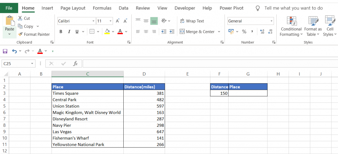
The formula to get the closest match in a data set is:
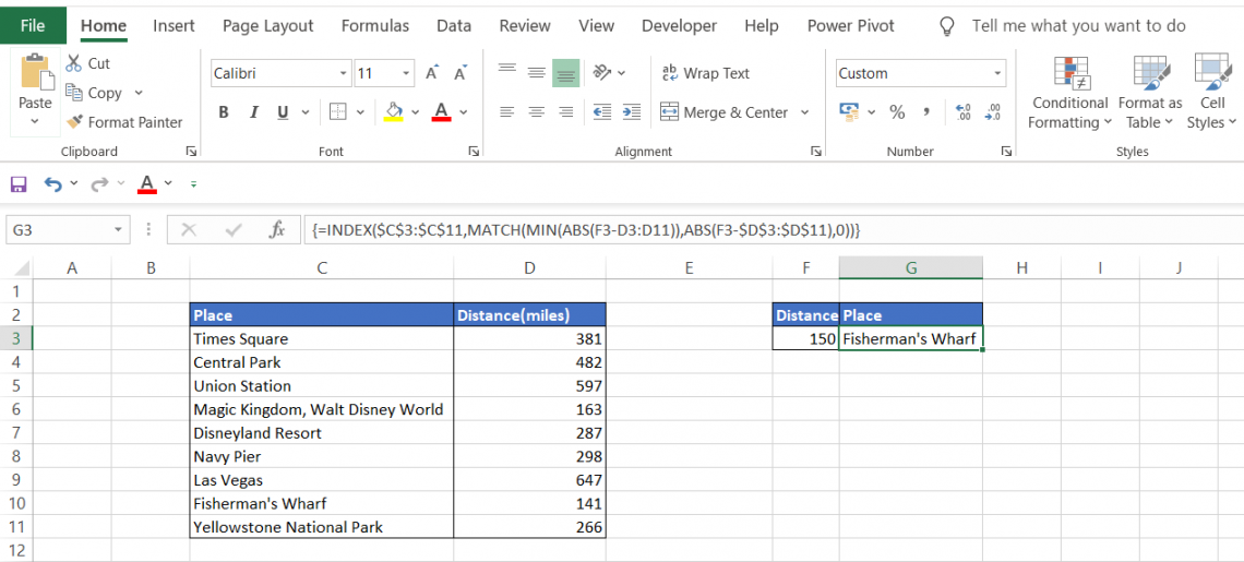
=INDEX($C$3:$C$11, MATCH(MIN(ABS(F3-D3:D11)), ABS(F3-$D$3:$D$11), 0))
Let's see how the formula works:
MIN(ABS(F3-D3:D11) gives the minimum distance (more or less) from the 150 miles that the car can travel. The absolute function converts the negative value into the positive ultimately giving the closest value.
In this case, the formula gives an array {231,332,447,13,137,148,497,9,116} consisting of the difference of 150 miles from the distances in column D.
The MIN function finds the smallest number from the array, 9 in this instance. Finally, the MATCH function pinpoints the location of the lookup_value, and the INDEX function gives the result as Fisherman’s Wharf which is 141 miles away.
Note
Since this is an array formula, you must press Ctrl + Shift + Enter in the cell to display the result, or Excel will give an #N/A error (except in Excel 365).
Bottom line
INDEX MATCH can do left lookups as opposed to VLOOKUP, which can only look for values to the right of the lookup_value.
The total length of a lookup criterion in VLOOKUP cannot exceed more than 255 characters, whereas INDEX MATCH works no matter how long the strings are.
Incomplete strings without exact match can also be used as lookup_values by the inclusion of wildcard characters to avoid #VALUE! Or #N/A errors, respectively.
If the data set contains thousands of rows along with the formulas, VLOOKUP gives results slower as compared to the INDEX MATCH formula.
The latter formula only assumes the column from which we expect the value, while the former includes the entire table resulting in a static column reference and increased processing time. This also increases the chances of errors in the values that we are expecting.
Since we specify particular columns in the INDEX MATCH formula for values, it allows us to add columns easily in the table without affecting the resultant lookup value.
The VLOOKUP function will shift the lookup results to either left or right depending on the location of the added column. This is one of the biggest advantages of this formula allowing the user to manipulate the data after inserting the formula in cells.

Free Resources
To continue your journey towards becoming an Excel wizard, check out these additional helpful WSO resources.


or Want to Sign up with your social account?