XMATCH Function
A Lookup and Reference function that returns the relative position of a specific item in a range of cells.


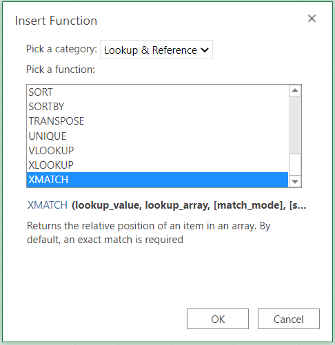
What is the XMATCH Function in Excel?
XMATCH is an inbuilt function in Excel 365 that returns the relative position of an item in a range of cells.
You must already be aware of the MATCH function and how, along with the INDEX function, it has become one of the most special formulas in the Excel community.
Considering the MATCH function's importance, Microsoft introduced the XMATCH function in Excel 365, which has similar capabilities but is more flexible and robust.
It can return the relative position from horizontal or vertical ranges, search for exact, approximate, or partial matches, and look from top to bottom or vice versa in the field of cells and gives the position 10.
-
Definition: XMATCH is an Excel 365 function for finding item positions in a cell range, offering enhanced flexibility.
-
Enhancements: Excel introduced XMATCH as an improved version of MATCH, providing options for exact or approximate matches and various search directions.
-
Syntax: XMATCH syntax includes lookup value, array, and optional parameters for match and search modes.
-
Usage Steps: To use XMATCH, specify lookup value and array, with optional parameters for customized search operations.
-
Examples: XMATCH can locate item positions, find adjacent values, and utilize different search directions.
Understanding the XMATCH Function in Excel
XMATCH is categorized as a Lookup and Reference function that returns the relative position of a specific item in a range of cells.
A successor to the MATCH function, the function offers some advantages to the user. These include specifying the match type to return exact or approximate matches (next smallest or largest value) and using the search mode argument, which allows you to look for a specific item in a first to last or last to first order.
The function is currently only available in Excel 365 and Excel 2021. All earlier versions do not support the use of this function. However, you can always head to Office 365 and run the Excel sheet to practice this new function!
Syntax for the XMATCH function
The syntax for the function is:
=XMATCH(lookup_value, lookup_array, [match_mode], [search_mode])
where,
- lookup_value = (required) the expected value we are looking for. For example, when looking for the stock prices, you use the ticker symbol for the stocks to look up their prices.
- lookup_array = (required) the range of cells considered for the lookup_value.
- match_mode = (optional) This argument specifies the type of match for the function. The different values that can be used for match_mode are:
| 0 | This is the default option that finds an exact match in Excel. The lookup_value must exactly match the value in lookup_array to return the value. |
| -1 | Returns the next smallest value if Excel does not find an exact match. |
| 1 | Returns the next largest value if Excel does not find an exact match. |
| 2 | This option lets you use wildcards, such as an asterisk( * ) and question marks (?) for partial matching |
search_mode = (optional) The search_mode specifies the way the function should look for the value in the lookup_array. The different arguments that can be used are:
| 1 | The function searches for the lookup_value in the lookup_array in the top to bottom direction. This is the default option if ignored. |
| -1 | Looks for the value bottom to top in the lookup_array |
| 2 | Used for a binary search where the lookup_array must be arranged in ascending order |
| -2 | Used for a binary search where the lookup_array must be arranged in descending order |
How to use the XMATCH Function In Excel
The first two arguments in the function are pretty straightforward. This section will focus mainly on the optional parameters that may or may not be helpful for you. The different steps that you need to follow to use the function are:
Step 1: lookup_value
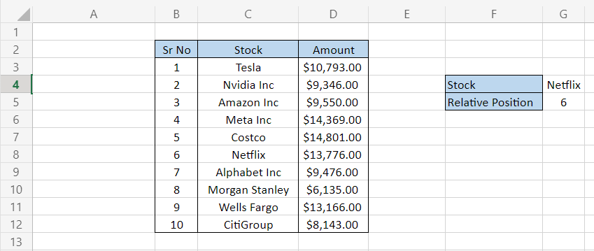
First, you begin with an equal sign (=) and type the function name to select the first argument, the lookup_value, as seen in cell G4 below.
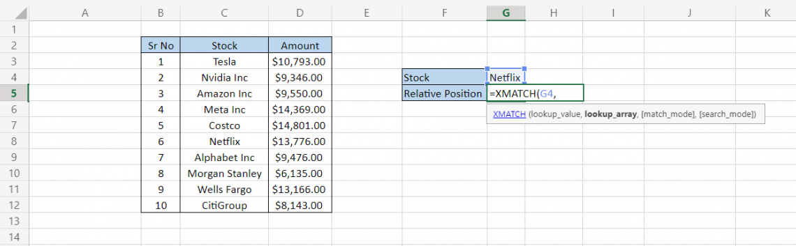
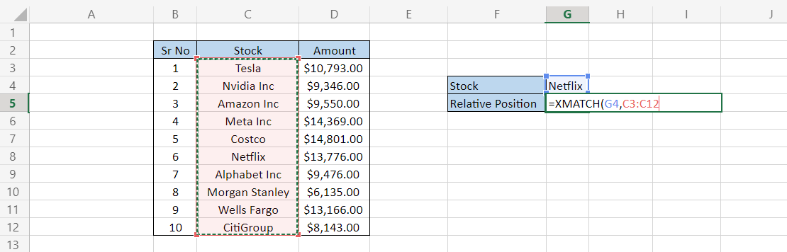
Step 2: lookup_array
The lookup_array is the range of cells in which we need to find the lookup_value. In this case, our lookup_array is from C3:C12, as illustrated below:
Step 3: match_mode
If you skip the match_mode argument, the value for the idea is 0, meaning that the function finds an exact match for the lookup_value.
If we use the formula
=XMATCH(G4, C3:C12,0)
we will get the result 6, the position of 'Netflix' stock in the array.
Well, what about the other argument's values? Assume that you have the ranks scored by each student, as illustrated below:
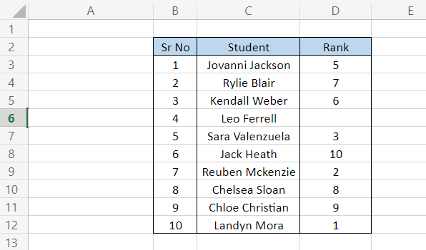
Let's say you need to find the position of one rank larger and smaller than 4 in the lookup_array D3:D12.
Assuming that there is no rank 4 in our data, we will use the formula
=XMATCH(G4, D3:D12,1)
to find the position of one level higher and
=XMATCH(G4, D3:D12,-1)
to find the position one rank lower than 4.
This will give us the results as follows:
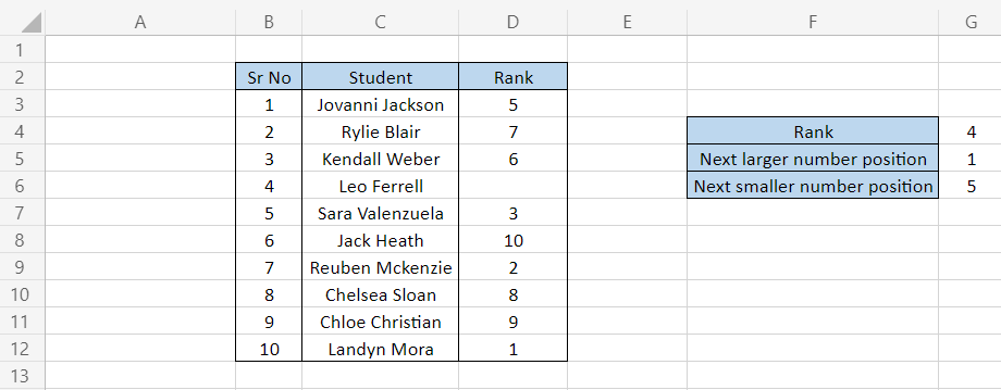
In cell G5, we can see that the position of the next highest rank to our lookup_value in our lookup_array is student 1, who had a status of 5. The next lowest level is equal to 3, whose relative position is 5, as represented in cell G6.
Yes, it can become a bit confusing when you are using the XMATCH function with numbers, but the pros outweigh this con.
Step 4: search_mode
The other optional parameter that the function consists of is search_mode. It is usually helpful when you need to find the position of the latest recurring lookup_value from the table.
Assume that you wrote journal entries for all the purchases and sales you made for the day. The spreadsheet is as illustrated below:
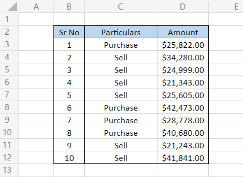
The default value for the search_mode is 1, which finds the value in the lookup_array from top to bottom.
By using the formula
=XMATCH(G4, C3:C12,0,1)
we will get the position of the first 'Sell' in the second cell in the lookup_array.
Similarly, if the search_mode value is -1, the function looks for the weight from bottom to top. So the formula becomes
=XMATCH(G4, C3:C12,0,-1)
and gives the position 10.

XMATCH Function Practical Example
Since the function supports partial match, you can find the position of such lookup_vales by using 2 as the argument for the match_mode parameter.
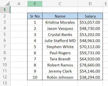
For example, suppose that you have this dataset consisting of employee names and their salaries:
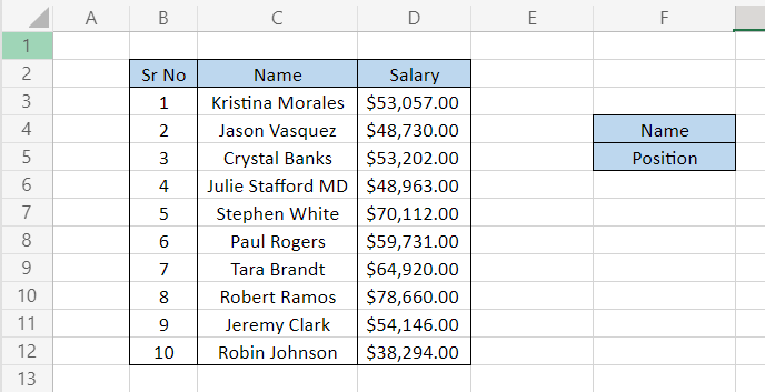
Suppose you need to find the position for 'Jason' in our table. Here, we will use the formula
=XMATCH(G4 &"*," C3:C12,2,1)
which will give you the result:
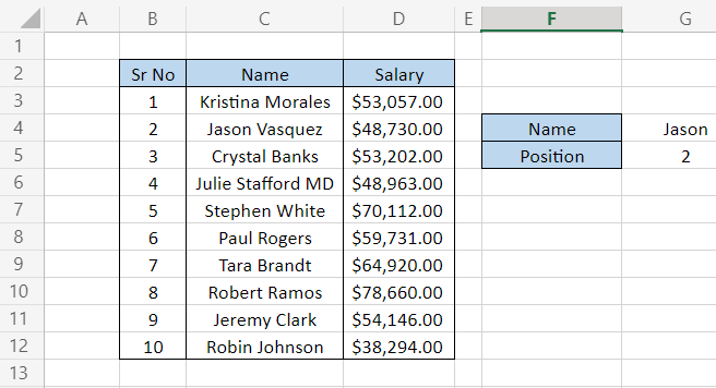
So, the position of Jason in our 'Name' lookup_array is 2. If you are not comfortable referencing values in the formula, you can also hardcode the lookup_value, which will update your procedure to
=XMATCH("Jason*," C3:C12,2,1)
BUT give you the same result.
XMATCH Function For Comparing two columns
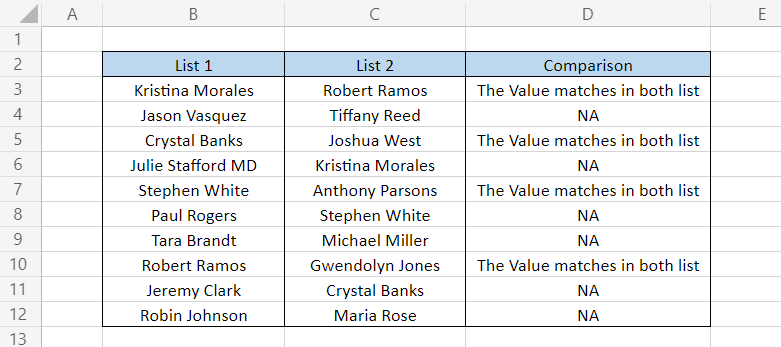
Suppose you have two columns of employee names, as illustrated below:
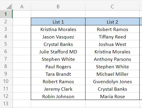
List 1 only includes employees with the company before COVID (2019), while List 2 covers employees currently working at the company (2022).
Now, if you want to find which employee has been working with the company for the entire period (2019-2022), we can use a combination of the IF, ISNA, and XMATCH functions.
If the lookup_value cannot be found, the ISNA function will return TRUE, as it detects the #N/A error. Based on this, we will set a logical expression using the IF process to produce a particular result if ISNA returns TRUE for an #N/A error or FALSE for no mistake.
The formula that we will use is
=IF(ISNA(XMATCH(B3:B12, C3:C12,0))
" NA," The Value matches in both lists"), which will give you the result:
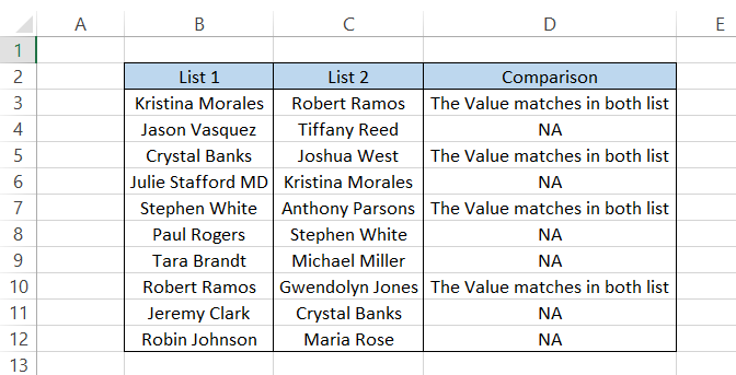
The value spills into the entire range since we used an array for our lookup_value. Therefore, if the value in List 1 does not exist in List 2, the result returns as "NA." Alternatively, if it matches, the formula returns "The Value matches in both lists."
An important thing to remember is that you will get the result in column D for List 1 since our lookup_value is range B3:B12.
For example, the value for B3 is 'Kristina Morales'. This value exists in both lists. Even though 'Kristina Morales exists in cell C6 in List 2, the comparison result will be for List 1.
Quite a helpful formula, right? Well, don't worry if you can't access Excel 365. You can use a similar procedure in Excel 2019 and older versions.
The formula becomes
=IF(ISNA(MATCH($C$4:$C$13,$D$4:$D$13,))
"NA," "The Value matches in both list") which will give you the same result:
Read more about the MATCH function in our dedicated article if you use an Excel version before Excel 365.
INDEX and XMATCH Function in Excel
The best use of the function is in combination with the INDEX function.
The INDEX-XMATCH combined function will return a value based on the relative position of a lookup_value in our referenced data. Then, this number will be used to search for information related to that data entry/column/row.
The syntax for the INDEX function is:
=INDEX(array, row_num, [column_num])
Where,
- array = (required) The range of cells that should return the required value. The subsequent row_num and column_num are optional if the array consists of only a single row or column.
- row_num = The rows from the array the returned value should be from.
- column _num = The column from the array the returned value should be from.
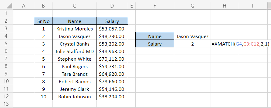
For example, suppose that you have the following dataset for employee names and salaries:
We will break our formula into two parts to understand it better. First, as usual, we will use the XMATCH function to find the relative position and then use the INDEX function to return a value based on the reference of that position.
To find the position for 'Jason Vasquez', we will use the formula
=XMATCH(G4, C3:C12,0,1)
This will give you the part of the lookup_value as 5.

If we want to return the salary for 'Jason Vasquez' with the result obtained from our XMATCH function, we will nest the consequence inside the INDEX function such that the formula becomes
=INDEX(D3:D12,(XMATCH(G4, C3:C12,0,1))
This will give you a salary of $48,730.00.
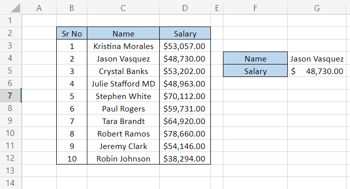
The range D3:D12 is the array from which we expect our result, based on the relative position of the INDEX function. The XMATCH function compared the index positions (1,2,3…) of all the values and finally returned the deal ($48,730) that matched position 2.
Check out our article on the INDEX MATCH formula to find out why we prefer it over VLOOKUP and how you can also use both functions best. MATCH performs a similar function as XMATCH, but it is outdated compared to its newer, upgraded counterpart.
XMATCH Function points to remember
Some of the points to keep in mind are:
-
When el is unable to find the lookup_value, it will return the #N/A error.
-
If multiple instances of the lookup_value exist in the lookup_array, Excel will return the first instance of that value depending on the search_mode argument set up in the formula.


or Want to Sign up with your social account?