ISNA Function

What is the ISNA Excel Function?

The ISNA function in Excel evaluates the given value and returns the result as TRUE if it is an #N/A Error and FALSE if not.

#N/A Error holds a crucial position in the error-handling process since it is one of the most prominent errors in Excel. The error means that the spreadsheet’s value is unavailable.

If you use the VLOOKUP or the INDEX MATCH function regularly, there is a high probability that you will end up with a #N/A Error if the value is missing.

Thus, considering the importance of #N/A Error and the presence of other errors such as #VALUE!, #REF!, #NUM!, #NAME? etc. Excel has bestowed the users with the ISNA that can easily identify the #N/A Error in Excel.

In this article, we will see what exactly is the ISNA error or what family of functions it falls under, along with a couple of examples to understand it better.

Understanding The ISNA Function

The ISNA is categorized as an Information function that checks if the referenced value is an #N/A Error to return the result as TRUE and FALSE if it is not.

For example, the function returns the result as FALSE if the cell has a numeric value, text strings, date/ time, or even boolean values. Similarly, if it is an error such as #NUM!, #VALUE!, #REF!, #NAME? then the function still evaluates to FALSE.

Only when the cell value is #N/A does the function evaluate TRUE. This makes it a really important tool for identifying errors in a given dataset.

where,

• value - (required) referenced value which will be evaluated for the #N/A error.

If you need to return a customized text string for the #N/A Error, then you can use the IFNA function, which can be said as a combination of ISNA and IF functions.

The function will first evaluate for NA error and then use the IF function to return a customized text string as a result based on the evaluation result.

Example of the ISNA function

When using it in Excel, it is easy to understand what one should expect from the function. Since the function isn’t that complicated, we will see a really simple example of how the function works and hop on to other alternatives in the Information function category.

Suppose we have the data as illustrated below:

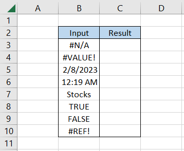
By using the formula =ISNA(B3) in cell C3 and dragging it down to cell C10, we get the result:

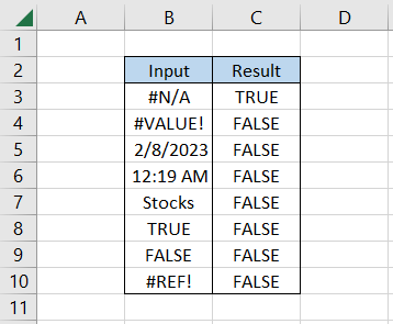
As you can see, our dataset comprises all the different types of values such as errors, date, time, text string, boolean values, etc., yet the function only returns the result as TRUE for #N/A Error.

What Is The IFNA Function?

The IFNA is categorized as a Logical function that returns a customized result if the referenced cell contains an #N/A Error.

If we break down the IFNA function, we understand it combines ISNA and the IF function. ISNA, as we know, evaluates the NA errors, whereas the IF function returns two different alternative results based on whether the condition evaluates to TRUE or FALSE.

However, IFNA can only return the customized result if it encounters the NA error. If there is no such error in the dataset, the function will return the same referenced value to the user.

The syntax for the IFNA function is:

=IFNA(value, value_if_na)

where,

• value - (required) the referenced cell containing the value which will be evaluated for #N/A Error.
• value_if_na - (required) customized value which will be returned in the presence of #N/A Error.

Let’s see an example to compare the IFNA versus the combination of ISNA and IF functions. Suppose we have the data as illustrated below:

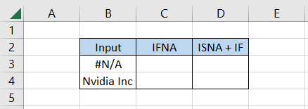
By using the formula =IFNA(B3,"This is NA error") in cell C3 and dragging it to cell C4, we get

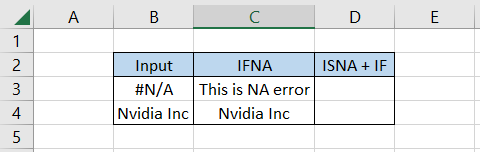
As you can see, the error value gives the customized text string, whereas when we had a hardcoded text such as ‘Nvidia Inc,’ we got the same result in column C. This would also apply to all the other error values apart from #N/A.

On the other hand, by using the formula =IF(ISNA(B3), "This is NA error", "This is not NA error") in cells D3 and D4, we get

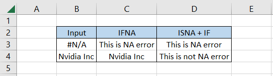
In this case, we can return two customized text strings based on whether the function is evaluated as TRUE or FALSE. Thus, you can use either of the two methods to evaluate the NA errors and return customized text strings.

Other error-capturing functions

Excel has an arsenal of other functions that you can use to capture errors, such as ISERROR, ISERR, and ERROR.TYPE etc.

The ability to identify errors and return the corresponding boolean value makes it an extremely important addition that every user must know.

In this section, we will see some functions considered ‘essentials’ if you intend to become an Excel wizard.

a. ISERROR

When you reference an error in the ISERROR function, it evaluates to TRUE, or the result will be FALSE. The different types of error values that you might encounter in Excel are #N/A, #VALUE!, #REF!, #NUM!, and #NAME? etc.

Capturing these errors makes it easier to rectify if there are any mistakes and return the correct values.

One of the most common errors is the #N/A seen using the lookup functions such as VLOOKUP. This is because if the value does not exist in the database, the function returns the result as #N/A.

For example, suppose you have the dataset as illustrated below:

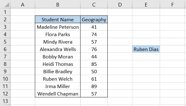
We need to find the test scores for Ruben Dias from the given dataset. Using VLOOKUP using the formula =VLOOKUP(E6,$B$2:$C$12,2,FALSE) in cell F6 gives the #N/A Error.

However, unlike the ISNA function, the ISERROR can capture other error values that might not have been possible with the help of the former.

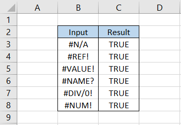
In the subsequent table, we use the formula =ISERROR(B3) in cell C3 and drag it down till cell C8, which gives the result as TRUE for all the error values.

b. ISERR

The ISERR function evaluates TRUE to all the error values except #N/A. This function works exactly opposite to ISNA, which evaluates FALSE to all the errors in excel #N/A.

If the requirement is to ignore the NA errors and understand the rest, then the best choice is to use the ISERR function.

Suppose we have the below dataset:

By using the formula =ISERR(B3) in cell C3 and dragging it down till cell C8, we get

As you can see, only when the referenced error is #N/A, the function evaluates to FALSE. For the rest of the values, the function evaluates to TRUE.

Thus, a simple inference can be made for all three information functions:

• ISNA - returns TRUE for only #N/A Error
• ISERROR - returns TRUE for all error values
• ISERR - returns TRUE for all errors except #N/A

c. ERROR.TYPE

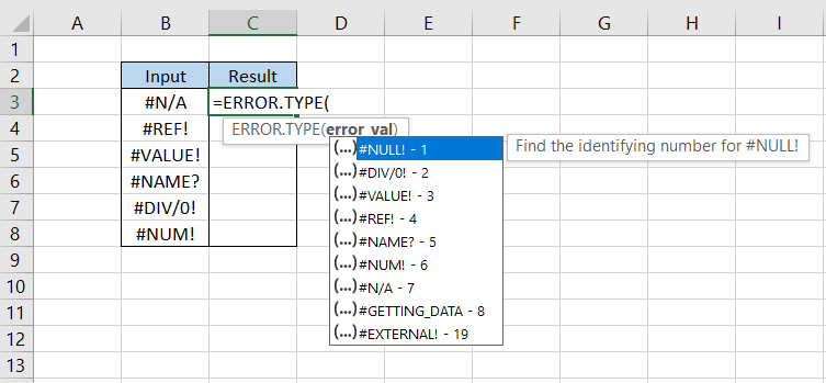
The ERROR.TYPE is a unique function in such a sense that it does not return a boolean value when it encounters an error but rather identifies the unique mistake and returns the corresponding integer value associated with it.

The integer values are already stored for these errors, and if such error-containing cells are referenced in the formula, the function returns the corresponding error value.

For example, #NULL! is stored as 1, #DIV/0 is stored as 2, #VALUE! as 3, #REF! as 4, #NAME? as 5, #NUM! as 6, #N/A as 7, etc.

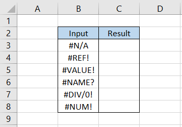
Suppose we have the data as illustrated below:

Thus, when we use the formula =ERROR.TYPE(B3) in cell C3 and drag it down till cell C8, which gives the result:

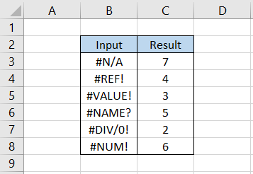
As you can see, each error has a unique integer assigned to them and does not overlap with the other values.

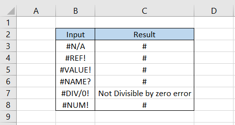
Thus, if we wanted to return a customized text string for a particular error, say #DIV/0! then we can use the combination of IF and ERROR.TYPE function.

The formula becomes =IF(ERROR.TYPE(B3)=2,"Not Divisible by zero error", "#"), which gives the result.

This way, you can improvise the formula to customize the result for different error values in Excel.

Researched and authored Akash Bagul | LinkedIn

Reviewed and edited by Parul Gupta | LinkedIn

Free Resources

To continue learning and advancing your career, check out these additional helpful WSO resources:

• HYPERLINK Function
• IFERROR Function
• IFNA Function
• INDEX Function
• LEFT Function