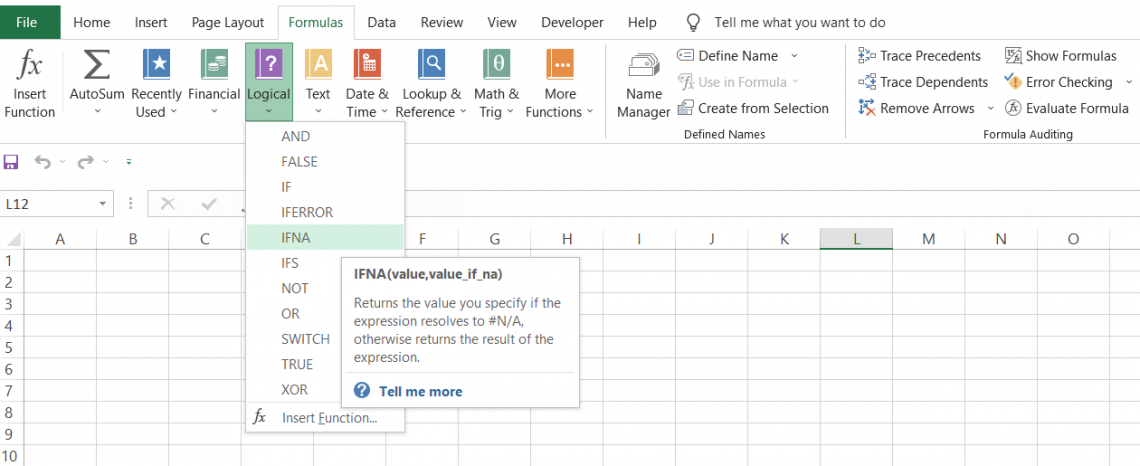
IFNA Function

What is the IFNA Function in Excel?

The IFNA function in Excel specifically traps the #N/A Error and returns a customized value specified by the user.

Let's agree that the #N/A errors are an absolute nuisance while working in Excel. So be it while using the VLOOKUP, INDEX-MATCH, or any other function that returns cell references, there is a high probability that you will see this Error.

We can't ignore these errors entirely as they can bring inaccuracy in the results that the Excel returns. However, going through all the cells individually and checking for errors can be pretty tedious, so the IFNA function comes in.

There are other errors, such as #VALUE!, #REF!, #DIV/0, #NUM!, #NAME?, and #NULL! , etc., but the specialty of the function is that it explicitly captures the #N/A Error and returns a customized result as input by the user.

This article will explore how you can handle the #N/A Error and why you see those errors in Excel.

Understanding the IFNA function

The IFNA is a logical function that evaluates a cell for #N/A error and returns a user-friendly message if the assessment returns TRUE. 

Suppose you need to lookup for 'Apples' in the range of cells consisting of values such as 'Mango,' 'Strawberry,' and Guava. When you use the formula =VLOOKUP('Apples,' B3:B5,1, FALSE), Excel returns the #N/A Error.

Why do we get the Error, though? Looking into the range B3:B5, we don't have a cell with the value 'Apples.' Since no such value exists in the range, it is Excel's way of conveying to the user that the deal is unavailable.

Another question that might arise to you is - Why does Excel not return the text not available? Again, the logic behind it is pretty simple. If you are working on a large amount of data, mainly text strings, the chances of overlooking the errors can be high.

Instead, Excel came up with the Number sign (#) that's added before the errors, so whenever you filter the text strings, you will always find those errors separated from the rest of the dataset.

IFNA Function Formula

=IFNA(value, value_if_na)

where,

• value = (required)reference to cell whose formula or expression needs to be checked for the #N/A Error
• value_if_na = (required)value that needs to be returned if #N/A Error is detected

How to use the IFNA Function in Excel?

When using the function, you must reference the cell with the error value and input the custom text as the other argument. So, for example, if the process captures the #N/A Error, the result would be a non-error value.

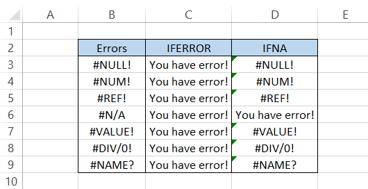
Let's say that you have different errors in Excel, as illustrated below:

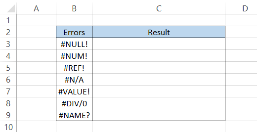
Then, you can expect the formula to identify only the #N/A Error in cell B6 of the table.

By using the formula =IFNA(B3, "You have value not available error!") in cell C3 and dragging it down to the cell C9, we will get the result:

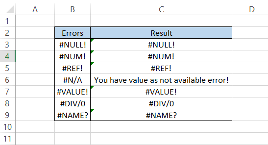
As you can see, all the other errors were ignored except #N/A, for which the function returned an alternate text string as "You have value as a not available error!". 

Another deduction we can make is that if the function cannot detect the #N/A Error, it will return the same error or value as our result.

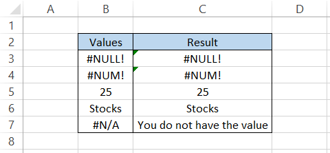
For example, let's say you have a combination of errors, numbers, and text strings in the data.

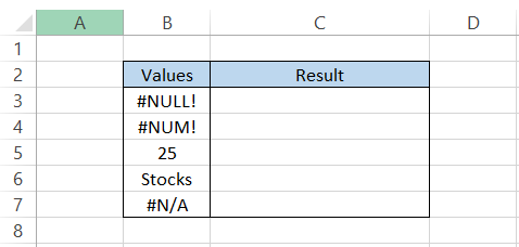
If you use the formula =IFNA(B3, "You do not have the value") in cell C3 and drag it down to the last cell, you will find that the same text strings and numbers are returned as a result.

The only difference we see is the #N/A Error, for which we get a customized text string - 'You do not have the value.'

Combination of IF and ISNA function

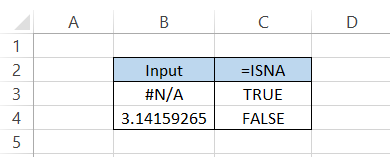
The function generally combines two essential parts - IF and ISNA. The IF process allows the user to make logical comparisons between two different values and return a value based on the comparison result, i.e., different values for TRUE and FALSE outcomes.

On the other hand, the ISNA error evaluates a cell for #N/A Error and returns the values TRUE or FALSE based on the outcome. The formula used is =ISNA(B3), which gives the result as:

Nest the result returned in cell C3 inside an IF function using the formula =IF(C3, "You have an error!"," "), and you will get the same result as the IFNA function. Alternatively, you can directly use the formula as =IF(ISNA(B3), "You have an error,") to give you the same result.

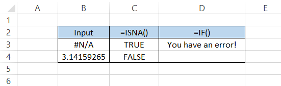
What is the advantage of this method? You can return another alternate text string/number if the comparison result is FALSE. The IFNA function will return only a single user-friendly value when it detects the #N/A error.

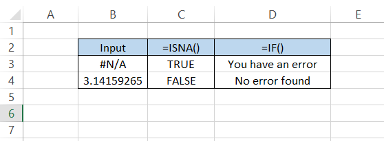
For example, no error exists in cell B4. Hence, when the combination of functions is used with the updated formula =IF(ISNA(B3), "You have an error," "No error found"), we get the result:

IFNA Function Examples

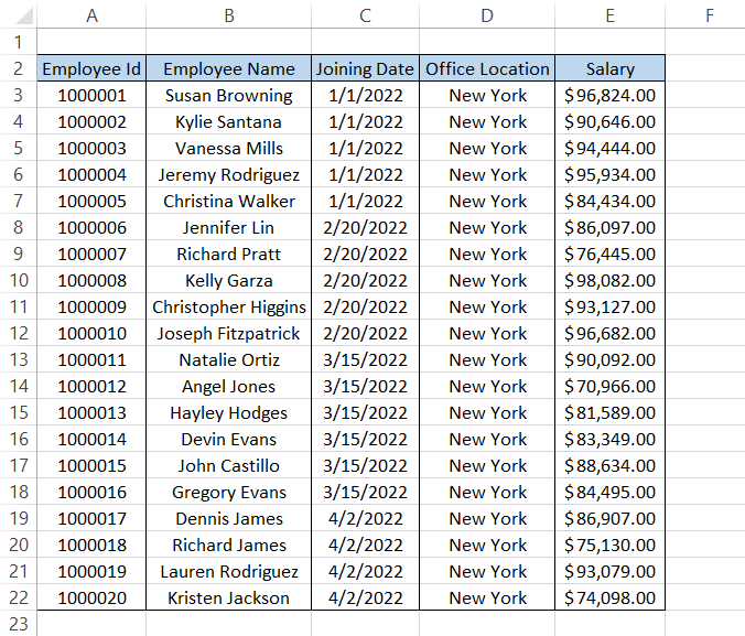
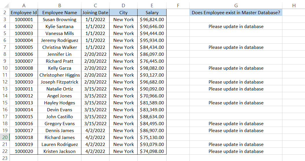
Suppose you have data for all the employees who joined your organization in 2022. First, you need to check whether the entries for all those employees are made in the master Employee database.

The data for the new joiners is in the 'Sheet1' of the workbook,' as illustrated below:

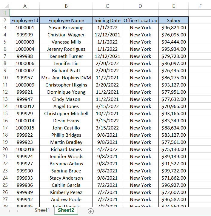
The master Employee database is present in the 'Sheet2' of the workbook as below:

To check whether the employee information exists in the master database, we will use the VLOOKUP function in 'Sheet1' using the formula, 

=VLOOKUP(A3,Sheet2!A2:E32,1,FALSE) 

This will give us the result as illustrated below:

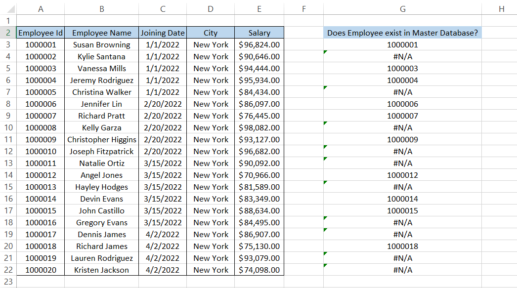
We have used the 'Employee Id' as the lookup_value, as they are likely to be unique compared to the 'Employee name' or 'Joining Date'. This is because the data for many new employees is not yet updated in the database. 

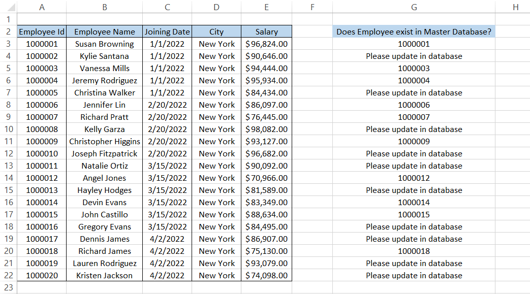
To make the Error more user-friendly, we can use the formula, 

=IFNA(VLOOKUP(A3,Sheet2!A2:E32,1,FALSE),"Please update in database")

This will give us the result:

You can also use the combination of IF and ISNA functions to return the same result. If those two functions were used here, the formula becomes 

=IF(ISNA(VLOOKUP(A3,Sheet2!A2:E32,1,FALSE)),"Please update in database","") 

Which gives a different result:

When the Error was detected, we chose to return the value as 'Please update in the database.' whereas when no error was found, we chose to return an empty string.

Whatever function you use in Excel has its pros and cons. For example, we could hide the existing results in the master database in this scenario. Hence, making our analysis more straightforward.

Example 2

The IFNA function can also be used to create a nested VLOOKUP that can be used to find a value through multiple spreadsheets.

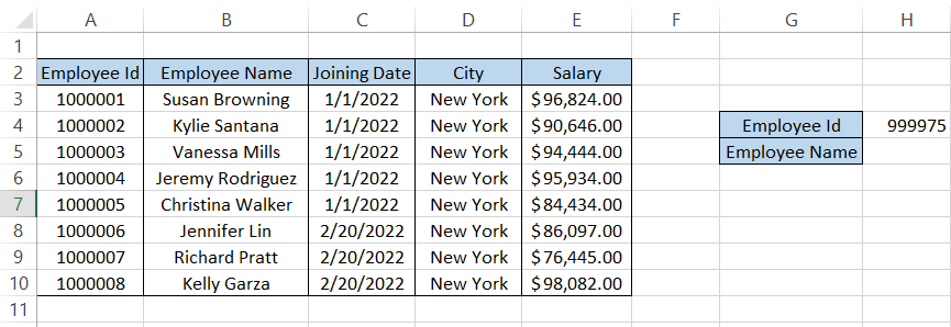
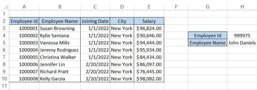
Let's say we need to find the employee's name with the Employee Id as 999975.

The data in Sheet1 looks as illustrated below:

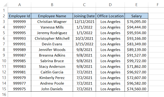
We have another spreadsheet, 'Sheet2,' that has all the employees working in the city of Los Angeles as:

The formula that we will use to return the name of the employee is, 

=IFNA(VLOOKUP(H4,A2:E10,2,FALSE),IFNA(VLOOKUP(H4,Sheet2!A2:E15,2,FALSE),"Employee does not exist in database")) 

This gives you the result as 'John Daniels'

The general idea behind the formula is that if VLOOKUP cannot find the value, the procedure will naturally return the #N/A error. 

Instead of an alternate message, we run another VLOOKUP in a different spreadsheet until it finds the value or ultimately gives us our customized text string.

You could have also used the IF statement or the IFERROR function here, and the formula would still work. This proves that Excel provides more than one way of doing something in Excel, but each method has its advantages and disadvantages.

IFERROR vs. IFNA

Now comes the time for debate. What's better - IFERROR or IFNA? The IFERROR returns an alternative result, usually text, when it detects all the types of errors.

The IFERROR has almost similar syntax. Which is

=IFERROR(value, value_if_error)

where,

• value = (required) a value, expression, cell expression, or a formula that needs to be checked for Error
• value_if_error = (required) value that needs to be returned if error is found

Suppose that you have several errors in the spreadsheet, as illustrated below:

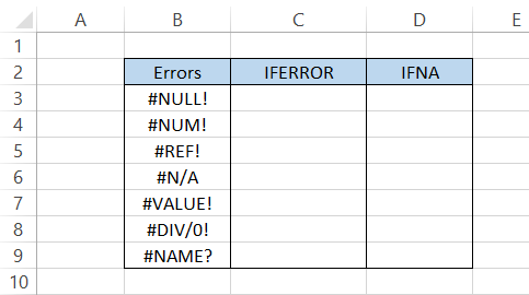
By using the IFERROR function, the formula will be =IFERROR(B3, "You have an error!"), which should give you a customized text string due to all the errors.

As you can see, the IFERROR function spares absolutely no error in its error-handling process and returns the result 'You have an error!' for all the mistakes.

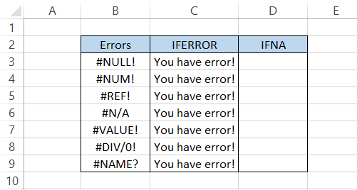
Let's use the IFNA formula for error handling and compare it with the IFERROR function. First, the formula will be =IFNA(B3, "You have an error!"), which will give you the result as illustrated below:

We get pretty contrary results where only the #N/A Error gets the customized text string while the rest of the errors are ignored.

We believe each Error should be handled individually rather than using the IFERROR function that returns the same result for everyone. 

You can use the function that best suits your purpose based on your view of the errors and what you intend to do with them.

Other error-handling functions

There are other error-handling functions that you can use to catch errors in Excel. Some of them are:

a) ISERR function

ISERR function evaluates and returns TRUE for all the types of errors in Excel, except #N/A. So, for example, if you have different errors in the spreadsheet and use the ISERR function, you will get the result below:

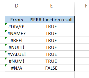
As you can see, by using the formula =ISERR(D3) in cell E3, we get the result as TRUE for all the errors except #N/A. You can use the combination of IF and ISERR to return the desired value based on the Error received, i.e., #N/A or everything else.

We have used to formula = IF(ISERR(D3)," Error is not #N/A," "Error is #N/A," which, if evaluated to TRUE, will return the result as "Error is not #N/A" or "Error is #N/A" for FALSE.

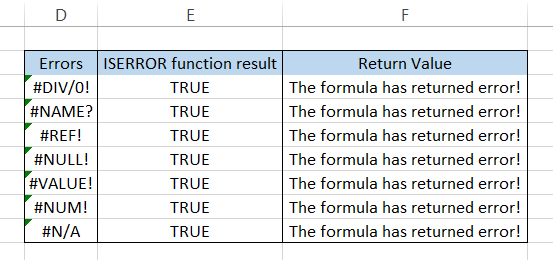
b) ISERROR function

The ISERROR will evaluate and return TRUE for all error types, including the #N/A. The combination of ISERROR and IF can be used as an alternative to IFERROR since, both ways, you will get the same result.

For example, by using the function =IF(ISERROR(D3)," The formula has returned Error!"," Not an error"), whenever Excel encounters a mistake, it will return the result as "The formula has returned Error! or return "Not an error" when the formula evaluates to FALSE.

c) ISNA function

While ISERR returns TRUE for all error types except #N/A, the ISNA function works exactly the opposite.

The ISNA function will return TRUE only for #N/A errors, while all the other errors will return the result as FALSE. So, for example, when you use the formula =ISNA(D3) for different errors in the spreadsheet, you will get the result:

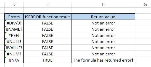
By combining the ISNA function with the IF function, the formula becomes =IF(ISNA(D3), "The formula has returned an error!", "Not an error") that further returns a custom text string as our result, as you can see for all the values in column F.

d) ERROR.TYPE

When you use the ERROR.TYPE function in Excel returns the number that correlates to the error value you might get while working on the spreadsheets.

For example, suppose you have the #NULL! Error in Excel, and you use the formula =ERROR.TYPE(C3) will return the result as 1.

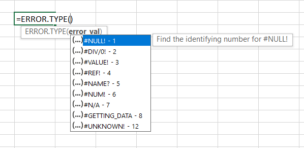
Based on the ERROR.TYPE result, you can use nested IF statements or IFS functions. If the spreadsheet has #DIV/0! You will get one outcome and another for a different error.

An important thing to note about ERROR. If Excel can find none of the errors in the referenced cells, the TYPE function will return the result as #N/A error.

Researched and Authored by Akash Bagul | Linkedin

Reviewed and edited by Parul Gupta | LinkedIn

Free Resources

To continue learning and advancing your career, check out these additional helpful WSO resources:

• FV Function
• PEARSON Function
• SEARCH Function
• SUBTOTAL Function
• YIELD Function