SUBTOTAL Function in Excel
One of the Mathematical Functions in Excel that allows you to return aggregate outcomes by performing different arithmetic operations.


What is the SUBTOTAL Function in Excel?
The SUBTOTAL function is one of the Mathematical Functions in Excel that allows you to return aggregate outcomes by performing different arithmetic operations, such as finding the sum, maximum value, minimum value, average, variance, etc., on the user-defined range.
The function is known for its versatility, allowing you to perform different tasks with a single function! This article will guide you on using the function for different arithmetic operations to improve your work efficiency.
As a financial analyst, you are expected to work on many calculations and number crunching, and a function like SUBTOTAL can make your life much easier.
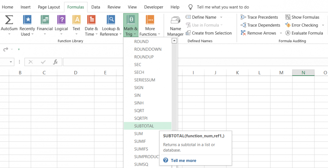
The function is categorized as a Math and Trigonometric Function that returns the aggregate for a given range of cells.
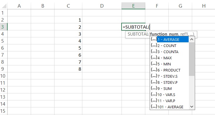
The function allows you to perform several arithmetic functions based on the number assigned to each unique role. For example, the number assigned to calculate the average of a range of cells is 1.
Similarly, if you intend to find the maximum value from a user-defined range, then the number you should select is 4.
You don’t need to remember the numbers and their corresponding assigned functions. Instead, when you type SUBTOTAL into the formula bar, it gives you a drop-down list to select the desired arithmetic operations.
- The SUBTOTAL function is an Excel Mathematical Function that performs calculations on a range of data while ignoring other subtotal functions within that range.
- Users provide two arguments to the SUBTOTAL function: the function number and the range of cells to be included in the calculation. It returns the subtotal based on the specified function number.
- Users might encounter potential errors when using the SUBTOTAL function, such as providing invalid function numbers or referencing cells with incorrect data and how to address them effectively.
- The SUBTOTAL function finds applications in financial modeling, budgeting, and forecasting, where summarizing and analyzing data is essential for decision-making and planning.
Why do we need to use SUBTOTALS?
But wait! Why do we have the same function, AVERAGE, but with different codes, i.e., 1-AVERAGE and 101-AVERAGE? If you scroll down, you will see that we have another series similar to 1-11 that begins from 101-111.
So the simple answer is - each has a different purpose. For example, the functions with the numbers 1-11 are used when you want to include manually hidden rows/columns into your calculations.
On the other hand, you can use the series 101-111 when you want to exclude the values from the hidden rows in your arithmetic operations.
The different types of arithmetic operations that you can perform using this function are:
| Function | Includes manually hidden rows | Excludes manually hidden rows |
|---|---|---|
| AVERAGE | 1 | 101 |
| COUNT | 2 | 102 |
| COUNTA | 3 | 103 |
| MAX | 4 | 104 |
| MIN | 5 | 105 |
| PRODUCT | 6 | 106 |
| STDEV | 7 | 107 |
| STDEVP | 8 | 108 |
| SUM | 9 | 109 |
| VAR | 10 | 110 |
| VARP | 11 | 111 |
The syntax for the function is:
=SUBTOTAL(function_num, ref1,..)
where,
- function_num = (required) a number corresponding to the functions in the list
- ref1 = (required) the cell or range of cells for which we need to determine the aggregate
You can use up to 254 additional optional ref arguments.
How to use the SUBTOTAL Function in Excel?
The function only takes in two arguments, but there can be variations to the result depending on what function_num your input in the formula. We will explore how the outcome would differ depending on what function_num argument you use.
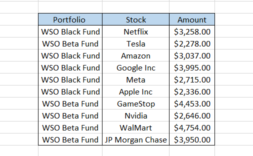
Assume you have the data in Excel as illustrated below:
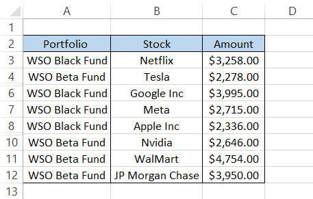
Since the stocks in rows 5 and 9 are currently sold, we will hide those two rows. The updated data looks as below:
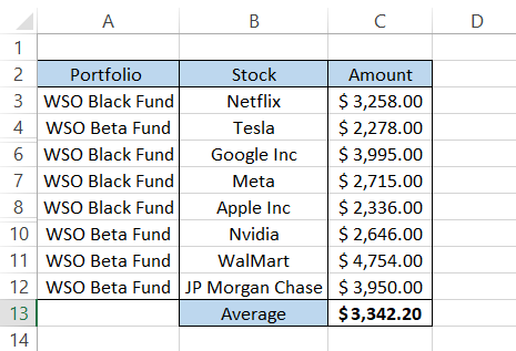
AVERAGE - 1
First, we will explore the effect of function_num 1-11 on our results. Of course, we already know that the result will include any manually hidden rows, which, in our case, are rows 5 and 9.
The formula we will use to find the average will be =SUBTOTAL(1, C3:C12). This will give you the standard for all the amounts, including the hidden rows, equalling $3,342.20.
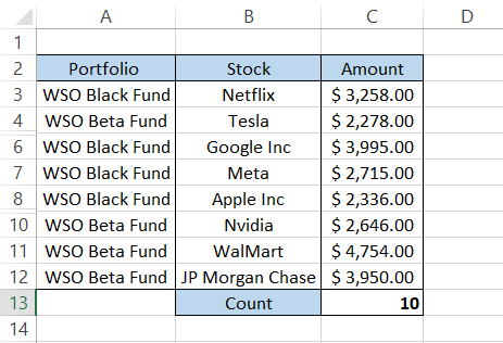
COUNT - 2
Next on the list is the COUNT function, which gives you the number of numerical values in your dataset.
The formula to find the count will be =SUBTOTAL(2, C3:C12), which will give us the result as ten, i.e., the total number of stocks in our dataset. However, if you use the function on text, you will not get the correct result.
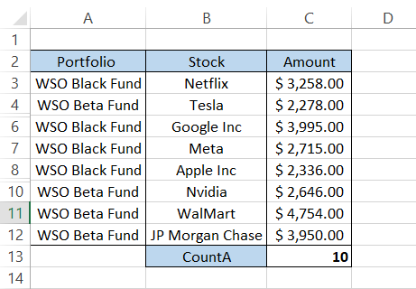
COUNTA - 3
The COUNTA function will count all the cells that contain a numerical value, text string, or a formula that returns empty rows or an error value. The only cells that would be excluded from the result will be the ‘truly empty cells.’
The function_num will change to 3, such that the formula becomes =SUBTOTAL(3, C3:C12), giving a result of 10. Even if the referenced range were B3:B12 or A3:A12, we would get the same result.
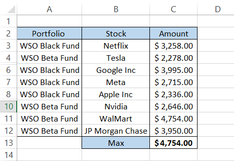
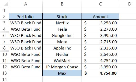
MAX - 4
The MAX function gives you the maximum value from the range of cells consisting of numbers. If you reference a range that consists of text, the MAX function skips those cells and excludes them from the result.
The formula becomes =SUBTOTAL(4,C3:C12). This will give you the maximum amount paid as $4,754.00 for Walmart.
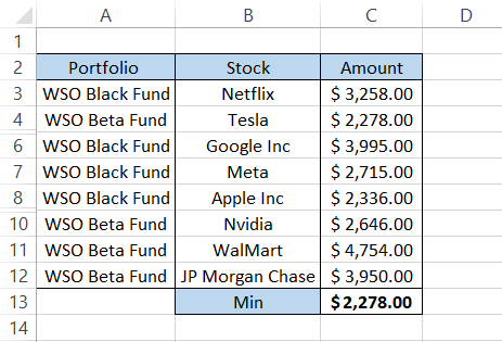
MIN - 5
The MIN function returns the minimum value from the range of cells consisting of numbers. The formula that includes the function_num as 5 becomes =SUBTOTAL(5, C3:C12), giving the result $2,278.00 for Tesla.

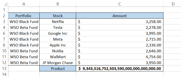
PRODUCT - 6
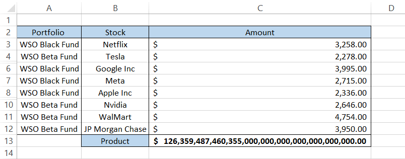
The PRODUCT function multiplies all the numbers in the given range of cells. By using the formula =SUBTOTAL(6, C3:C12), we will get the product for all the amounts in the range C3:C12 as:
STDEV - 7
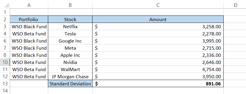
A standard deviation helps the user understand how much the values in the dataset deviate from the mean/average value. If the result returned is small, all the values lie around the mean value, while if the result returned is large, the values in the dataset lie farther away from the mean.
By using the formula =SUBTOTAL(7, C3:C12), we will get the standard deviation as $891.06, which means ‘most’ of the values in our dataset fall within the range of $3,342.20 (mean) +/- $891.06.
STDEVP - 8
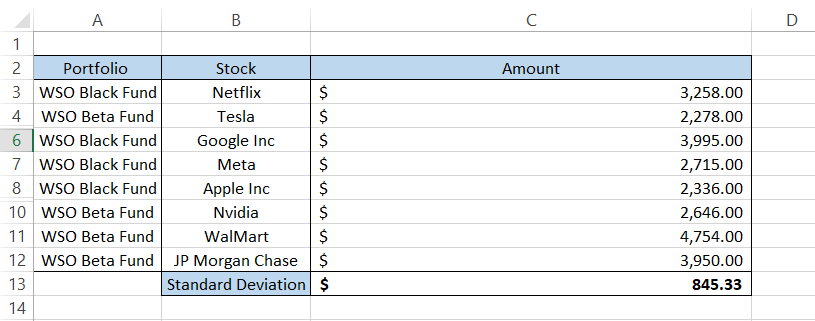
Generally, when you have a sample of the data, we use the STDEV function. However, if you have a dataset representing the entire population, then the best choice of the formula is STDEVP.
The formula =SUBTOTAL(8, C3:C12) will give you the result as illustrated below:
SUM - 9
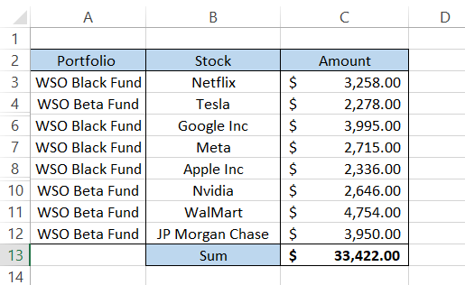
Finally, comes the function beloved by all Excel users: the sum function calculates the total of all the values in the range of cells.
By using the function_num as 9, we can activate the SUM function such that the formula =SUBTOTAL(9, C3:C12) gives us the result of $33,422.00
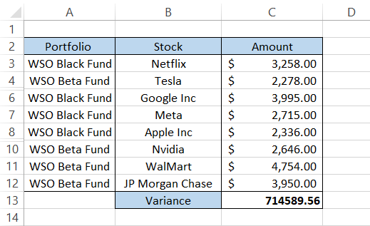
VAR - 10
The VAR (variance) function measures how spread out the values are in our dataset. Variance can also be calculated as the square of the standard deviation. Our standard deviation was 891.06, whose square, i.e., 891.06 x 891.06, will give us the result of $79,3987.90.
If you use the formula =SUBTOTAL(10, C3:C12) for VAR, you will get approximately the same result in Excel:

VARP - 11
Just like we had the standard deviation for an entire population, we also have a variance for data considered a total population.
Previously, our standard deviation for the population was $845.33, which, if squared, gives us the result of $71,4582.80. This is our variance for the dataset, considering it is data from every unit in the population.
If we use the formula =SUBTOTAL(11, C3:C12), which is the variance for population, we get an approximately similar result:
By using the function_num between 1 to 11, the function includes all the rows in our result even if they are manually hidden data in Excel.

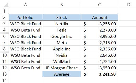
AVERAGE - 101
Since we already know what different arithmetic operations you can perform, we will see the effect of those functions by using the function_num from 101 to 111.
Remember, rows 5 and 9 are still hidden in our dataset since those stocks were recently sold from the portfolio.
The formula we will use is =SUBTOTAL(101, C3:C12), which will give us the result of $3,241.50 as opposed to $3,342.20 when we used function_num as 1.
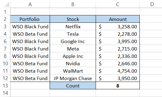
COUNT - 102
Using the formula =SUBTOTAL(102, C3:C12), we will get the result as 8, a difference of two from when function_num was 2, meaning our manually hidden rows are excluded from the impact.
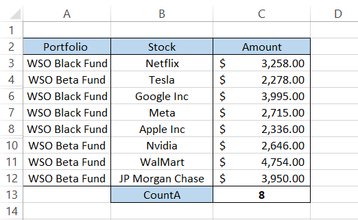
COUNTA - 103
The formula to count the cells containing the numbers, texts, and errors, excluding hidden rows, is =SUBTOTAL(103, C3:C12), which will give the result 8.
MAX - 104
The maximum value can be calculated using the formula =SUBTOTAL(104, C3:C12), giving $4,754.00. Since the row with the maximum value was not hidden, we got the same result.
MIN - 105
Another result equal to its counterpart, =SUBTOTAL(105, C3:C12), is what we got using the function_num five.
PRODUCT - 106
The product will change since we exclude two rows from our result. The formula will be =SUBTOTAL(106, C3:C12), giving us:
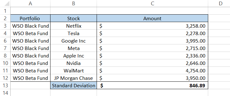
STDEV - 107
The standard deviation, excluding the hidden rows, will be calculated using the formula =SUBTOTAL(107, C3:C12), giving the result:
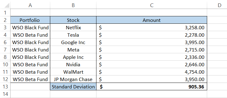
This means most of the values lie between the range $3241.50 (calculated using function_num as 101) +/- $905.36.
STDEVP - 108
The standard deviation of the entire population, excluding the hidden rows, will be calculated by the formula =SUBTOTAL(108, C3:C12) to give the result:
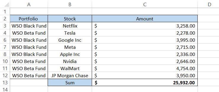
SUM - 109
Finally, the part that would be the most important for you as a financial analyst. You might sometimes need to hide rows in your data and calculate the sum for loan amounts or total portfolio amounts in Excel.
Rather than hiding the rows and copying the data into another spreadsheet, you can hide the rows and use the formula =SUBTOTAL(109, C3:C12), giving you the result:
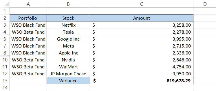
VAR - 110
Again, the VAR (variance) function measures how spread out the values are in our dataset. Variance can also be calculated as the square of the standard deviation.
Our standard deviation using the code 107 was $905.36, whose square, i.e., 905.36 x 905.36, will give us the result of $819,676.73.
Using the formula =SUBTOTAL(110, C3:C12) gives us a roughly approximate value, as illustrated below:
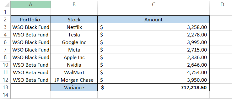
VARP - 111
Last but not least, the formula to calculate the variance of the entire population, where hidden rows are ignored, is =SUBTOTAL(111, C3:C12), giving the result:
Using SUBTOTAL from the Excel ribbon
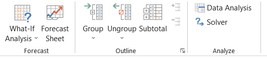
There is another way you can use the function in Excel. It is by clicking on the Data tab and hovering the mouse over the Outline section that you will find the function, as illustrated below:
-
Select the entire dataset and click on the function
-
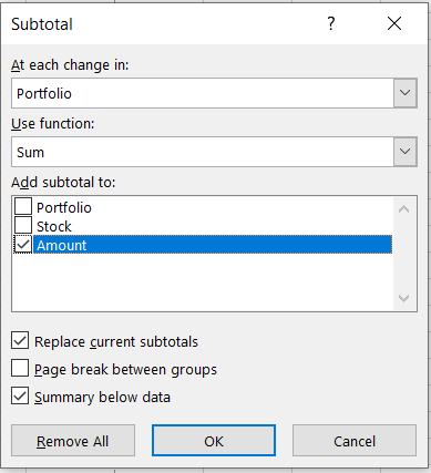
The dialog box that will open up will look like this:
-
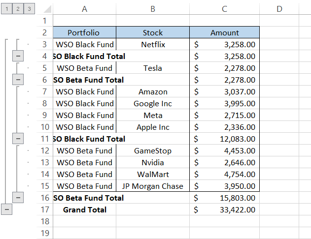
Here, the function allows us to create summary rows with aggregate values. Once you click on OK, you will get the result:
-
In the result, we can see that the table is aggregated based on the portfolio. Once the portfolio changes, the aggregate value changes. This is a more appropriate version of the subtotal function. The choice is really up to you for what method to use, but either way, you are bound to get the result.
Tips for the SUBTOTAL function
Some of tips are:
-
When the function_num is between 1-11, the hidden rows are included in the result of the function.
-
The hidden rows are excluded from the result if the function_num is between 101-111.
-
When you use the filter function to ‘filter’ the table by specific criteria, the formula considers all the rows of the table in the result irrespective of what function_num you use in Excel.


Free Resources
To continue learning and advancing your career, check out these additional helpful WSO resources:


or Want to Sign up with your social account?