IF Statement Between Two Numbers
How to Combine IF with AND functions


Excel is a powerful spreadsheet software that can be used for many different purposes. One of the most common functions in Excel is the IF function, which allows you to compare numbers and make decisions based on those comparisons. The IF function is one that all advanced Excel courses will cover - for example, Acuity Training's course in London. This article will outline how to use IF with the AND function in Excel.
What is an IF Function?
An IF function in Excel is a logical function that compares two numbers or data types and returns a value for a TRUE result and another for a FALSE result.
For example, suppose the marks required to pass in English as a subject is 35. We would then have to set up an IF statement such that if the marks are more than 35, the value returned will be “Passed”, else the value returned will be “Failed”.
To set up an IF statement in Excel, you need the following:
- The cell where you want the result to appear
- The comparison operator (i.e., >)
- The value to compare against (i.e., A1)
- The value to compare against if the condition is met (i.e., B1)
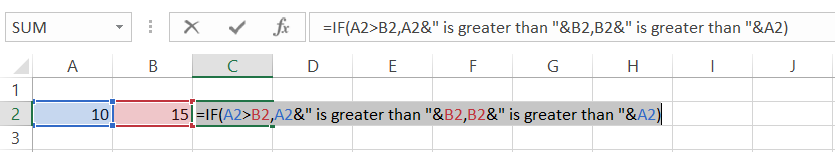
For example, say you have A1 and B1 values as 10 and 15, respectively. Your IF statement would look like this: =IF(A2>B2,A2&" is greater than "&B2,B2&" is greater than "&A2). This would calculate whether A1 is greater than B1 or vice versa.
Syntax for IF function
The syntax for the IF function is:
=IF(test expression, value if condition is TRUE, [value if condition is FALSE])
where,
Test expression = the condition that you want to test
value if the condition is TRUE = The value that is returned by the function if the condition turns to TRUE
value if the condition is FALSE = The value that is returned by the function if the condition turns to FALSE
Comparison Operators
The logical operators play an essential role in representing the different conditions used in the If statements. These comparison operators help us compare numbers and strings and perform complex conditions assessments. Listed below are the operators you can use while using the If statement.
| Condition | Operator | Example | Description |
|---|---|---|---|
| Equal to | = | =IF(A1=20,TRUE,FALSE) | If the numerical value in A1 cell is equal to 20, the result will return as TRUE or otherwise as FALSE |
| Not equal to | <> | =IF(A1<>20,TRUE,FALSE) | If the numerical value in cell A1 is not equal to 25, the result will return as TRUE or otherwise as FALSE |
| Greater than | > | =IF(A1>20,TRUE,FALSE) | If the numerical value in cell A1 is greater than 20, the result will return as TRUE or otherwise as FALSE |
| Less than | < | =IF(A1<20,TRUE,FALSE) | If the numerical value in cell A1 is less than 20, the result will return as TRUE or otherwise as FALSE |
| Greater than or equal to | >= | =IF(A1>=20,TRUE,FALSE) | If the numerical value in cell A1 is greater than or equal to 20, the result will return as TRUE or otherwise as FALSE |
| Less than or equal to | <= | =IF(A1<=20,TRUE,FALSE) | If the numerical value in cell A1 is less than or equal to 20, the result will return as TRUE or otherwise as FALSE |
Simple IF examples (Using dates)
Suppose that you work at XYZ fund. All the buy/sell trades are reconciled at the end of the day for those whose settlement date falls on that day. For example, assume that the following trades were undertaken from 24th Jan 2022 to 26th Jan 2022.
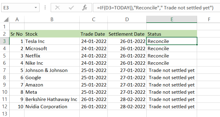
On 26th Jan, you open Excel to find that trades made on 24th display the status as “Reconcile”. To do this we have used the formula =IF(D3=TODAY(),"Reconcile"," Trade not settled yet").
Since we have used the TODAY() function, which fetches the current date, it runs every day on the opening of the file, which means that if the settlement date is “Today”, it will be labeled as ‘Reconcile”. But wait, you open the file and find that our previous trades that were already reconciled show the status as “Trades not settled yet”.
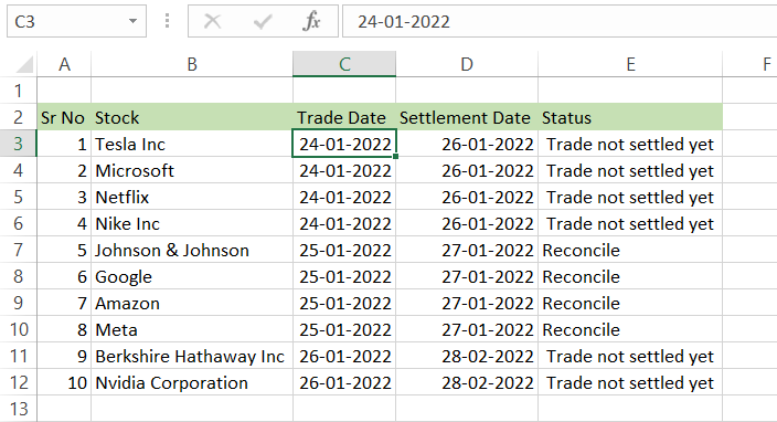
Well, worry not! All you need to do is add another If statement or make a nested if, which in this case the formula used will be =IF(D3<TODAY(), “Reconciliation Done!”, IF(D3=TODAY(), “Reconcile”, “Trade not settled yet”)). Then, when you drag the formula in the entire range, the result you will get is as follows:
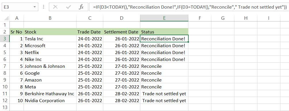
This way, you will always be up to date with the status of the trades before the day begins!
Also, we will discuss the nested IF in the next section of our article.

Nested IF’s
Using one IF function inside another allows you to test additional conditions, which increases the number of potential results for your test expression. These nested IFs are easier to read and debug, which helps take proper action on the dataset based on the combination of conditions.
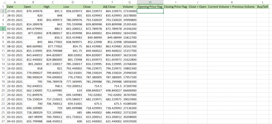
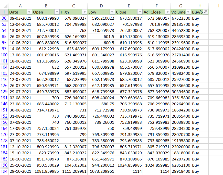
For example, let’s assume that you have Tesla Inc (NASDAQ: TSLA) OHLC data for the past year extending up to 255 rows in your spreadsheet. We need to determine buy signals based on four conditions:
- Condition 1 - Current opening price should be higher than the last opening price
- Condition 2 - Current closing price should be higher than the last closing price
- Condition 3 - If conditions 1 and 2 are satisfied, the closing price should be higher than the opening price.
- Condition 4 - If condition 3 is fulfilled, the current volume should be greater than the previous volume.
NOTE
We have added headers in the table to help understand our conditions better. We expect either TRUE or FALSE as a value in each cell before the Buy signal is generated in column L. If any condition returns as FALSE, our If statement will end and return the value as an empty cell in column L.
This is the same example for which we have written a similar VBA code that incorporates IF statements and For loop. You can check that article here.
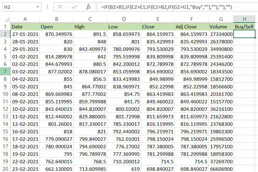
Here, we are using the formula =IF(B2>B1, IF(E2>E1, IF(E2>B2, IF(G2>G1, "Buy", ""), ""), ""), "") in column H. The nested if statements check the conditions in a way where it will move onto the next condition only if the preceding condition is met, failing which it will return the result as an empty cell. Copy the formula up to the last row in the ‘Buy/Sell’ column.
Filter the data using the keyboard shortcut Alt + H + S + F and select the criteria as ‘Buy’ to remove the blanks in our dataset created due to our conditional statements.
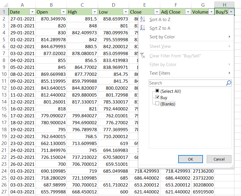
This is how our spreadsheet will look like with a total of 35 buy signals to invest in Tesla this past year (this is not investment advice, but rather an example to display how conditional statements work. You don’t have to HODL, YOLO, or buy high, sell low on your trades! Check out WSO Alpha to get exclusive trade alerts ;) )
Previously, Excel had a limit of a maximum of 7 nested If for its 2003 and lower version. However, in the modern versions beyond Excel 2007 to 2019, you can nest up to 64 If statements together. It is not advisable to use them anywhere near those numbers since a lot of reasoning goes into making the nested If statement works correctly. Even if it works, there might be a chance that it breaks the logic before going through all the conditions.
Any other person working on the same excel spreadsheet might not understand the logic of the conditions if there are no properly documented SOPs or instructions. Remember, the idea is to simplify the work and not complicate it. So at the slightest hints of trouble, try taking a different approach to tackle the problem at its root.
How to use the IF with AND function in Excel
So assume that your nested IF formula works perfectly fine in the spreadsheet. But you still need to check whether all the cells are non-empty(we have deleted values in some cells to demonstrate the formula), and if so, only then give the ‘Buy’ signals in our spreadsheet.
For this, we can build the IF AND statement that evaluates more than two conditions in the same formula. Only when all the formula conditions are met will the result return as TRUE or FALSE.
This is what our spreadsheet currently looks like:
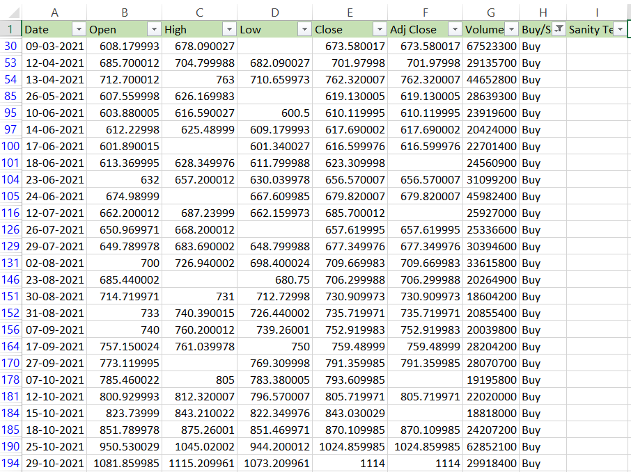
We have added an additional column in our spreadsheet as ‘Sanity Test’ to determine the integrity of our dataset. Here we use the formula =IF(AND(B30<>"", C30<>"", D30<>"", E30<>"", F30<>"", G30<>"", H30 = "Buy"), "All parameters exist!", "Error")
This formula checks whether all the cells from column B to G in your spreadsheet are non-empty and if the values in column H are equal to ‘Buy’. If all the criteria are met, the value displayed in the cell will be “All parameters exist!”. After copying the formula up to the last row, our spreadsheet looks as follows:
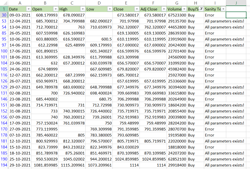
This shows that our formula works, after which values can be added to the empty cells.

NOTE
The IF statement in Google Sheets allows you to test conditions and return one value if the conditions are true and another value if the conditions are false.
How to use the IF and OR function in Excel
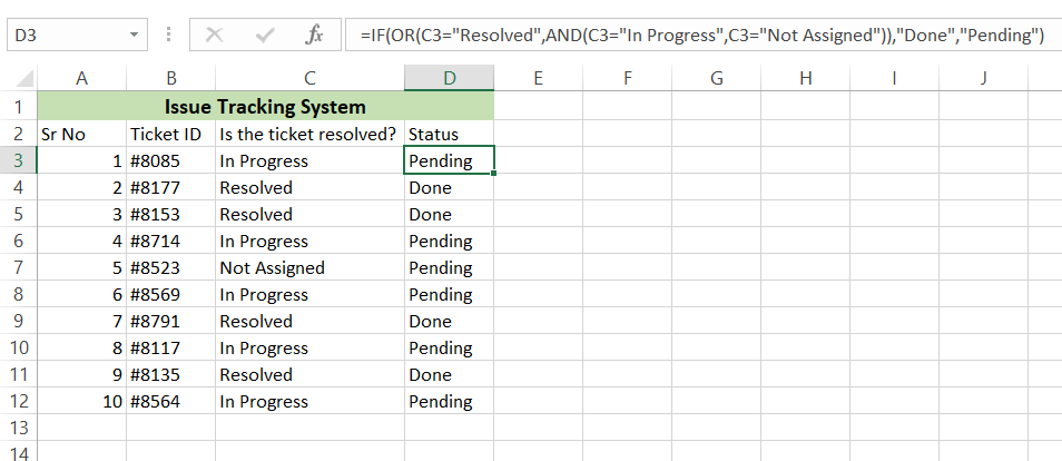
Let’s say that an IT support company needs to track its ticket system efficiently. The status of the ticket will be displayed in column D as either “Pending” or “Done” based on the parameters in the C column.
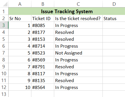
Here we have three different values, i.e., ‘In Progress’, ‘Not Assigned’, ‘Resolved’ in column C. If the value is either of the former two, we will get the result as ‘Pending’, or else the status will be ‘Done’.
We have used the formula =IF(OR(C3="Resolved", AND(C3="In Progress", C3="Not Assigned")), "Done", "Pending") by incorporating the OR function. We have also used the AND function since the result for either one means the ticket is still pending to be resolved. Our final result in the spreadsheet is as follows:
Once you understand the basics of how the If statements work and how to incorporate the AND/OR functions you can play around the formulas and make things work as per your necessity.
You can add a total of 255 conditions in the OR function in Excel versions 2007 and above, while in versions 2003 and below, the maximum limit is 30 conditions.
IF statement using strings
One of the advantages of using the If statement is that it does not recognize case sensitivity by default. That means it will identify ‘EXCEL’ and ‘excel’ as the same values.
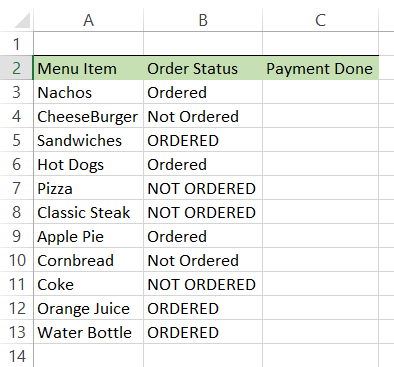
For example, assume that the customer orders the following items from the menu at the restaurant. However, the order status appears in the upper case due to some glitch.
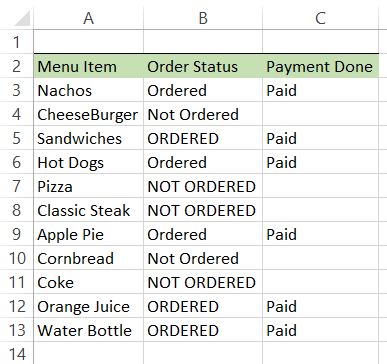
However, when you use the =IF(B3= “Ordered”, “Paid”, “") formula in column C, you will see that Excel identifies the values as case insensitive, i.e., for every status either as ‘Ordered; or ‘ORDERED’, the value in the Payment Done column will be ‘Paid’.
Any other values will leave the cell empty as per our defined conditions. So this is what our spreadsheet looks like after getting the result:
If you intend for the If statement to be case sensitive for your result, then you must use the EXACT function in your statement. For example, by using the formula =IF(EXACT(B3, “Ordered”), “Paid”,” “), Excel will only display the result ‘Paid’ for the cells in column B, which have value as ‘Ordered’.
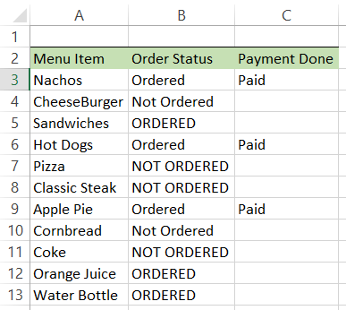
This way, you can match the values exactly in your spreadsheet. Remember to enclose your text values in the quotation marks or reference them in a different cell, or the function will give you an error.
Practical Example #1
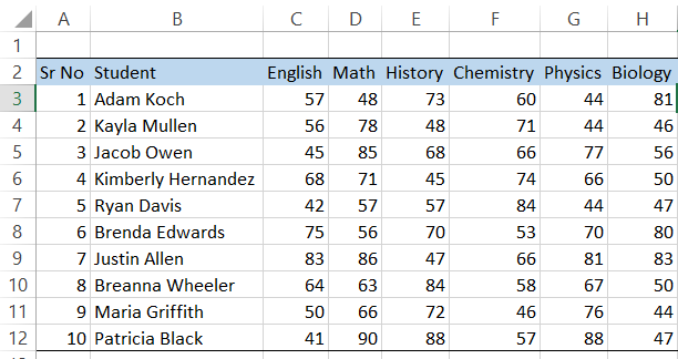
Assume that the teacher needs to categorize the results of the students in their class into three different categories - Excellent, Good, and Satisfactory.
Each student gives a total of 6 exams for 600 marks out of which they must score greater than 430 marks for ‘Excellent’, greater than 380 but less than 430 for ‘Good’, and anything less than 380 would fall in the satisfactory category. The dataset looks as follows:
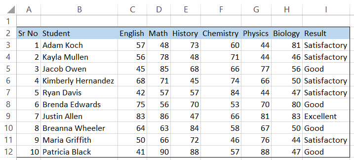
Here, we have used the combination of If statements and the Sum function that checks the total marks scored by each student and compares them with our categorization criteria. The formula used in cell I3 is =IF(SUM(C3:H3)>430, "Excellent", IF(SUM(C3:H3)>380, "Good", "Satisfactory")).
So when you drag the formula up to the cell I13, you will see the following result:
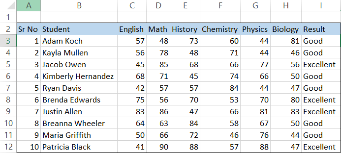
Similarly, you can also use the average function along with the if statements such that the average of scores obtained by students if greater than 65 will result in getting an ‘Excellent’ result. In contrast, an average below 35 will result in ‘Good’. The formula used will be =IF(AVERAGE(C3:H3)>65, "Excellent", IF(AVERAGE(C3:H3)>35, "Good", "Satisfactory")).
This is what our spreadsheet should look like:
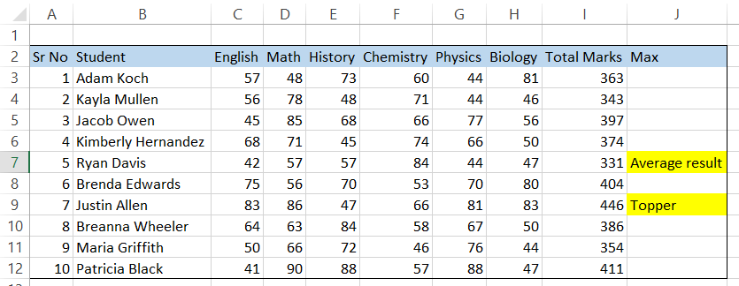
Another function that can be used along with IF statements are the Min/Max functions. The Min function lets you find the smallest number from the group, while the Max function will give you the biggest number.If you frame your formulas correctly, either of these functions will work wonders while working on a data set.
In case you need to find the student scoring the highest and the lowest total, you can use the formula =IF(I3=MAX($I$3:$I$12), "Topper", IF(I3=MIN($I$3:$I$12), "Average result"," ")) which will result in:
Practical Example #2
So assume that you are reconciling two different values in one of the tasks assigned by your manager. It’s normal to get abbreviated values for some commonly used terms such as ‘Yes’, ‘No’, ‘Adjustable Rate Mortgage’ as ‘Y’, ‘N’ or ‘ARM’, respectively. If you compare such values with their counterpart using the If statement, it might not give you the value you are looking for.
Let’s look at an example to help understand it better.
As we can see from the data above, we receive data from two sources:
- The internal source
- The loan servicing company
Since there might be thousands of loans, it is necessary to reconcile both the sources and track any discrepancies to check the integrity of the data.
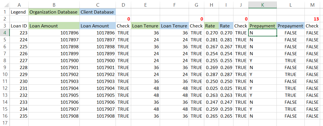
All of our data matches except those in the ‘Prepayment’ columns. We see that in internal sources, it is represented as ‘Y’ and ‘N’ if the loan borrowers have or have not made any prepayments on their obligation. However, in the loan servicing source, its values are represented as TRUE or FALSE.
As expected, comparing both the cells using =K4=L4 will give a FALSE value. So how to overcome this issue?
Here, you can use a combination of the If statement and OR logical function to give you either value based on the conditional statement. We use the formula =IF(OR(K4&L4="NFALSE", K4&L4="YTRUE"), TRUE, FALSE).
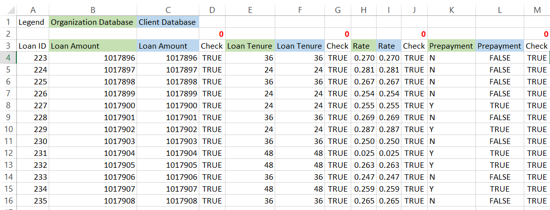
By concatenating both the values and then using the OR logical function to give a TRUE value, this is how our spreadsheet looks like:
In short, you can always play around with different functions to help you achieve the desired results. Furthermore, different functions have different applicability, and including them in the conditional statements can work wonders in your data analysis.
Other Important Functions that can be used in IF statements
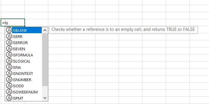
The Is prefixed functions return the value as TRUE or FALSE based on the value they evaluate. It can either check even/odd values, whether a blank cell exists in the spreadsheet, or return the condition as TRUE if errors exist in the dataset.
Instead of just flagging the cells as TRUE or FALSE, you can incorporate them in your conditional If statements to give you two different results based on the boolean values.
The different Is functions that you can use are:
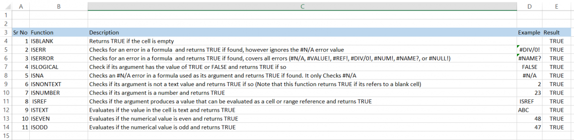
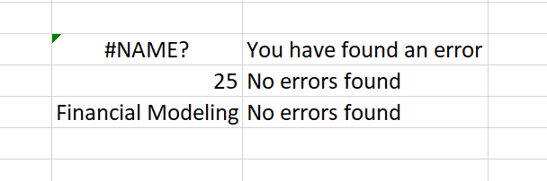
The Is prefixed functions such as ISNA, ISERR, ISERROR can be used for error handling, i.e., to give alternate values, in case errors are generated in excel. For example, we have used the formula =IF(ISERROR(G6), “You have found an error”, “No errors found”) to check if any errors exist in the database. If the error exists, the value will return as “You have found an error,” or else it will be “No errors found”
More on Excel
To continue your journey towards becoming an Excel wizard, check out these additional helpful WSO resources.


or Want to Sign up with your social account?