IFS Function
Returns a value that meets the first TRUE condition


The IFS function is a logical function that lets you run multiple conditions and return a value that meets the first TRUE condition. They are similar to the nested IF in their functionality, however, they are much easier to use than their counterpart. It was introduced in 2016 and is available to use in Excel 365 and Excel 2019.
- IFS allows you to check multiple conditions and returns the first value where the condition is TRUE.
- It is easier to use than nested IF statements for multiple conditions.
- The syntax is =IFS(condition1, value1, condition2, value2, etc.) with up to 127 condition/value pairs.
- IFS is more flexible than SWITCH since you can use comparison operators like <,>,= in the conditions.
- IFS works well with data validation to create dynamic drop-downs that display descriptions based on the selected value.
What is the IFS function?
The IFS function will let you evaluate multiple conditions that are easier to write and read to return a value based on the first TRUE result. If there are three conditions, and the second condition returns TRUE, then it marks the end of the logical function.
Think of it as a three-way battle between the conditions where the second condition comes out victorious. For example, you have a list of 10 students along with the marks scored in different subjects.
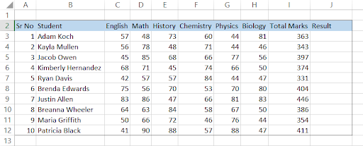
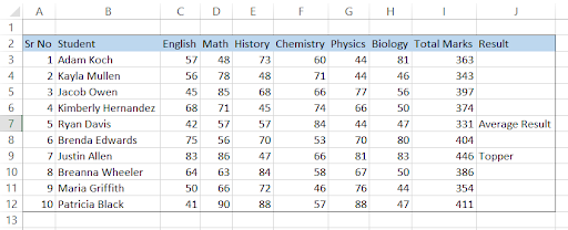
If you need to determine which student has scored the highest and the lowest total marks, you can use this function by using it in the formula =IFERROR(IFS(I3=MAX($I$3:$I$12), "Topper", I3=MIN($I$3:$I$12), "Average Result"), "") which will give the following result:
Note
If the function is unable to return TRUE for all the logical functions, it will return a #N/A error. It does not have a default value in case all the conditions return FALSE.
Syntax for IFS function
The syntax for the logical function is:
=IFS(logical_condition_1,Value1[logical_condition_2,Value2]...,[logical_condition_127,Value127]
where,
- logical_condition_1 = The required condition which is then assessed by Excel to check whether it is TRUE or FALSE
- Value1 = The value that is returned when the logical_condition_1 is TRUE.
Note
You can use up to 127 logical conditions in this function that evaluates to TRUE or FALSE. Apart from the first condition, the rest are all optional which depends on your preference while working on a particular dataset.
How to use the IFS function?
You do not need to make extra efforts while using the IFS function. However, you should be sure about the conditional statements that you need to include in the function. The conditions will use different comparison operators such as equal to (=), less than (<), more than (>), less than or equal to (<=), more than or equal to (>=), and not equal to (<>).
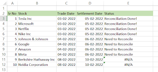
Assume that you have the trade book for stocks that need to be reconciled on the T + 2 day.
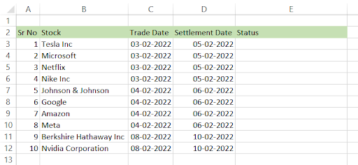
Now if the settlement day is today, the status will be “Need to reconcile”. Anything else before and after the settlement date will be either “Reconciled” or “Trades pending for settlement” respectively.
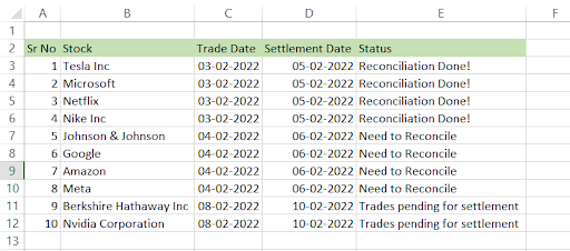
The formula used here will be =IFS(D3<TODAY(), "Reconciliation Done!", D3=TODAY(), "Need to Reconcile", TRUE, "Trades pending for settlement"). The formula essentially says that if the settlement date is less than today, the trades are already reconciled and if the settlement date is today then the trades must be reconciled today with what is present in the holding of the portfolio.
Remember that the IFS function does not return a value if all the conditions return false. So we have added a TRUE at the end of the function so that if none of them are triggered to return a result, the final result will be obtained which is “Trades pending for settlement”.
This is similar to the Else part of the If Else statement that is used to ensure that we do not receive the #N/A error in Excel.
After copying the formula in column E, our spreadsheet looks like this:
If you would have instead used the formula =IFS(D3<TODAY(), "Reconciliation Done!", D3=TODAY(), "Need to Reconcile"), i.e., by ignoring the Else part of the formula, your table would have looked as follows:
As the conditions do not evaluate TRUE for the settlement dates in rows 11 & 12, the function returns the #N/A error.
IFS function vs Nested IFs
In practice, IFS is the simplified version of the Nested IFs formula. Deeply nested ifs are difficult to understand and predict whether it will run the correct code or not. Even if one of the conditions doesn’t work, it affects the whole formula. Then comes the error handling part and if these nested statements are complicated you will have a hard time maintaining the code.
Hence, IFS is preferred by most analysts while working on financial data. Let us check out an example that shows how the formula differs for both IFS and the Nested Ifs.
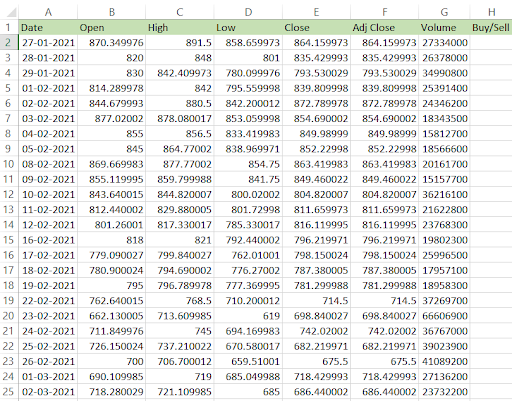
Assume that you have the historical data for Tesla from the previous year to date. You need to make an Excel model that helps you to generate ‘Buy’ signals in case certain parameters of the historical data are fulfilled.
The conditions upon which the model is based are:
- Condition 1 - The current opening price should be higher than the last opening price
- Condition 2 - The current closing price should be higher than the last closing price
- Condition 3 - If conditions 1 and 2 are satisfied then, the closing price should be higher than the opening price.
- Condition 4 - If condition 3 is fulfilled, the current volume should be greater than the previous volume.
This is what your Excel spreadsheet dataset looks like:
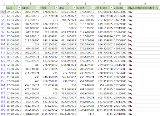
Now Tony, an Excel expert who has been working in your organization for the past 12 years, creates a nested if formula that evaluates the conditions and generates the “Buy” signals in column H. He uses the formula =IF(B30>B29, IF(E30>E29, IF(E30>B30, IF(G30>G29, "Buy", ""), ""), ""), ""). This means that if any of the conditions returns FALSE, the cell will remain empty. Only on fulfillment of all criteria will the value be “Buy” column H. This is how the spreadsheet looks after filtering the data:
Since Tony is an expert, he has no problem reading the code. But imagine an intern who joins the organization and is asked to tweak the formula or add an additional parameter. The issues that the complicated code will cause are obvious.
We believe that as our readers, YOU prefer to work smart. You are now well aware of the IFS function and use the formula =IFS(AND(B2>B1, E2>E1, E2>B2, G2>G1), "Buy"). What was once quite complicated, you have made it silly simple. The AND logical function ensures that only if all the conditions are fulfilled, will the cell show the value as “Buy”.
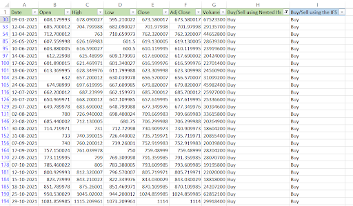
We understand that some of you might not like the sight of the #N/A errors all over in column I. To remove those errors you can follow two methods: Either use the Else part in the function, i.e., which changes the formula to =IFS(AND(B3>B2, E3>E2, E3>B3, G3>G2), "Buy", TRUE, "") which will return an empty cell or use the IFERROR function which will help to return the desired value in case of #N/A error.
The formula including the IFERROR function will be =IFERROR(IFS(AND(B2>B1, E2>E1, E2>B2, G2>G1), "Buy"), "").
IFS vs Switch
The SWITCH function will check if a particular value exists in a list of values and return the first matching result. The syntax for the switch function is:
=SWITCH(expression, value1, result1, [default_or_value2, result2]). The expression argument can be a referenced cell, text, number, or the boolean value (TRUE or FALSE).
However, the drawback of using the SWITCH function is that you cannot use comparison operators in the expression. This likely makes it quite a rigid function to use while working on a large dataset.
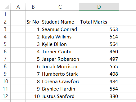
Let’s see an example of how the SWITCH works and evaluate its drawbacks. Below is the dataset for the students along with the total marks they have scored in their exams. The teacher must determine their grades based on certain parameters given below:
- If the total marks are greater than 550, the student will get an A grade.
- If the total marks are greater than 500, the student will get a B grade.
- If the total marks are greater than 450, the student will get a C grade.
- If the total marks are greater than 420, the student will get a D grade.
- If the total marks are greater than 400, the student will get an E grade.
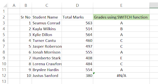
The formula that we use to grade the students based on the switch function is =SWITCH(D3, 563, "A", 514, "B", 564, "A", 460, "C", 497, "C", 555, "A", 408, "E", 484, "C", 554, "A", 411, "E"). Think of it similar to an array, where the values which are available in an array would return a value and the rest would give an #N/A error.
In our data table, the total marks for Justus Sanford do not match, i.e., the table shows the total marks as 380 while the formula shows the marks as 411. This is the rigidity of the switch formula.
The input will be your expected output or else an error. So if you have comparatively less data, and want to avoid mistakes at all costs then SWITCH is an excellent function to use. The table using the SWITCH formula looks like this:
On the other hand, the formula to grade the students based on IFS is =IFS(D3>550, "A", D3>500, "B", D3>450, "C", D3>420, "D", D3>400, "E"). Using this, no matter what marks are scored by the students, if they fall within the constraints we will get the correct graded value as illustrated in the table below:
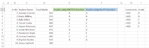
We would always prefer formulas that give us more flexibility while working which is why IFS is our preferred function over SWITCH.
Practical Example #1
If you intend to build dynamic Excel spreadsheets, then the combination of data validation tools with IFS works wonders.
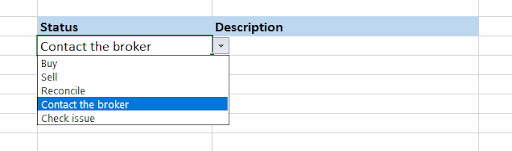
For example, we have five statuses such as ‘Buy’, ‘Sell’, ‘Reconcile’, ‘Contact the broker’ & ‘Check issue’ as a drop-down list from the data validation tool. To add them, press the keyboard shortcut of Alt + A + V + V, click on the Data tab, and then on the Data Validation tool which will open the Data Validation dialog box as below:
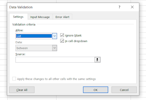
Here, add all the status in the source input box or you can also reference the cells from the spreadsheet, i.e., C6:C11 which contains the values for the validation tool. Once you press OK, your cell will have the drop-down list as shown below:
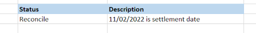
Now, you can add descriptions to each status using the IFS function such that any status selected using the validation tool will display the correlated description (when the value_if_true condition is fulfilled).
The formula that you will be using is =IFS(F4="Buy", "You have bought the stock", F4="Sell", "You have sold the stock", F4="Reconcile", TEXT(TODAY(), "dd/mm/yyyy") & " is settlement date", F4="Contact the broker", "Ticket has been generated and looked into", F4="Check issue", "Tech team has been notified").
Yes, the formula looks big at first glance but once you look into it, it's just repeating or going into a loop. The formula checks if the cell F4 has a specific value, say ‘Buy’, and then returns the corresponding value if found true else goes onto the next status.
As you change the status in the spreadsheet, the description changes as well. You can use the same formula and link the data validation list to different cells such that a change in status causes a ripple effect in the entire spreadsheet or the linked cells.
Note
TODAY() function is used in conjunction with the TEXT function since you will commonly encounter date formatting issues along with strings (dates will be represented as serial numbers, for eg. - 44606). To avoid this, we format the date using the “dd/mm/yyyy” which returns our date in the correct format.

More on Excel
To continue your journey towards becoming an Excel wizard, check out these additional helpful WSO resources.


or Want to Sign up with your social account?