Documenting Excel Models Best Practices

Documenting Excel Models Best Practices

Due to the large and complex nature of financial models created on Excel spreadsheets, it is of utmost importance that the models are accompanied by comprehensive documentation that will help users maintain and audit them efficiently. This article looks at some of the best practices for the documentation of financial models that are created in Excel.

Documentation might not be as exciting as working on the financial models, but it is nonetheless a crucial part of any project. Suppose you are on leave, vacationing in the beautiful Bahamas, and things go astray in the financial model you made. Who are they going to blame? It will be your head in the guillotine (well, speaking metaphorically) as the company would want a scapegoat for the mess. Documentation acts as insurance to speak on your behalf when you are not around to explain how your financial model works.

Model structure

Before creating any new model on Microsoft Excel, it is recommended to step aside and visualize how data will flow through it. A financial model consists of three main components - inputs, processing, and output. It is essential to understand the inputs, expected outputs, and how data flows and changes from input to output. This ensures that the model is organized from the get-go with the relevant worksheets, datasets, manual pages, etc.

The modeler should provide all information available about the inputs while avoiding redundancy. Also, the inputs must be differentiated from the outputs using formatting, color coding, etc.

Data validation is a powerful tool that checks the quality of the input data before processing it into the output. The comments help record different smaller details of the model and improve its overall efficiency. Lastly, one of the most important things to consider is how complex your financial model should be.

For example, if you are tasked with performing a discounted cash flow (DCF) analysis to advise senior management regarding potential acquisition opportunities in the market, it will be based on simple assumptions. More complicated DCF models would be prepared for the final acquisitions, tailor-made to the company.

Version control

A large data set will result in complex models, leading to multiple versions of the same model. Confusion with version control is very common among Excel users.

Imagine that you worked on a financial model only to later receive its latest version from Bob in Block D. Such things frequently happen, considering how demanding and iterative the financial modeling process is at the top private equity and investment banking firms. You can easily lose track of important work files if they are not documented properly.

It can often be difficult to obtain the correct version of Excel documents when more than one person is working on them. The first question that pops into our mind is “Is this even the latest version of the file?” Such situations can be avoided by following the best version control practices.

Consistent naming system

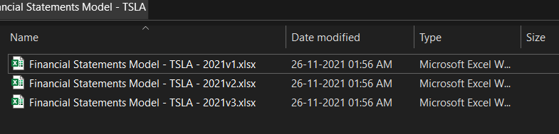
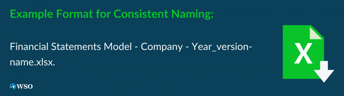
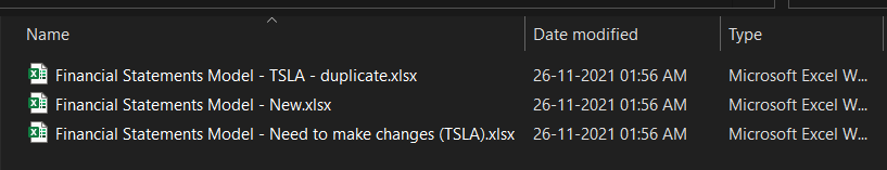
A consistent naming system helps identify the latest version of the file when sorted by name in the concerned folder. The last modified date can sometimes be untrustworthy as it may accidentally reset while working on an older version, especially when the changes are saved. Hence, an example of a consistent naming system format is “Financial Statements Model - Company - Year_version-name.xlsx.”

Two types of naming systems are used to avoid confusion about the correct Excel file version - the three-point edition system and the date version system.

The three-point edition system - Based on software programming, this system assigns numbers in increasing order as the developments are made on the file. Any file starts with the 1.0.0 version with the first number indicating the major changes made in the Excel file, while the second and third numbers are reserved for small and minute changes, respectively.

While working on large projects, it is always advisable to follow a three-point system to distinguish between the major changes, for example, “Financial Model - TSLA - 2021v2.1.0.xlsx”, while a single number version might be enough for small projects.

Master “version” Excel sheet

Documenting “versions” in a separate Excel sheet is another way to avoid the hassle of multiple file versions. This sheet will include the version name and the changes that were incorporated while working on it. This way, an analyst can always revert to the preceding versions of the Excel model. A master sheet is used to document versions in two different ways - a master sheet in the same workbook or a master Excel sheet in a separate workbook.

If the first or last spreadsheet is used as a ‘versions’ sheet, it falls under the first category. An example might explain this better.

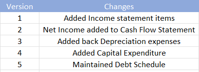
Suppose you have to make a financial statement model for a company, and you add all the items on the income statement. Due to some reason, you need to postpone working on it and save and close it after documenting the changes in the master sheet. When you work on it again later, you can add a new spreadsheet and copy all the data from the previous one to further work on the cash flow statement.

This way, any major changes will always be on a new spreadsheet in the same Excel while preserving the older changes. The Excel master sheet would look as below after some time where the version also represents the spreadsheet number.

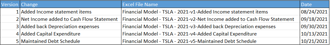
The separately prepared master sheet will document the changes and the name of the files created along with the changes on the particular date. This is particularly helpful if your Excel model consists of vast amounts of data and can freeze or even stop responding, thereby acting as a liability. If by chance, you have entered incorrect data, you can always refer to the master Excel sheet, return to the major change, and start working your way up from it.

What to avoid

It’s always the best practice to avoid common terms like ‘new version,’ ‘duplicate,’ or ‘final.’ An example of a file naming format that must be avoided is “Financial Model - TSLA - 2021 - duplicate2”. If filenames include a proper description, they are easier to find, especially if they are held on a shared server. Also, a saved file should follow a proper hierarchy if it contains different levels of data rather than adding common terms to the end of the file, as it can create confusion among the people working on it.

Most people also like to avoid blank spaces in file names as a personal preference and rather use a dash or underscore. If files with blank spaces are stored on web servers, it replaces the space with “%20” – making such files harder to find. Thus, using a dash or snake case (with underscores) enhances readability.

A company-wide consistently managed naming system using proper descriptions to describe the file’s contents ensures the application of good naming convention practices. It helps the company in the long run.

Below are a few ways you shouldn't be naming your Excel files.

Titles for Worksheets, Charts, and Tables

We always find it difficult to retrieve files if they are not saved systematically using a proper naming convention. Organized files make it easier to navigate through other people’s work. A good naming system ensures that a person knows the file’s contents without opening it.

For example, a file named "Financial Model - TSLA - 2021v2.1.0.xlsx" tells the user that it is the financial model for the company, Tesla, for the financial year 2021, and the version of the file is 2.1.0. As opposed to this, names like “Untitled.xlsx” or “New Microsoft Excel Worksheet.xlsx” do not give much information about the contents of the Excel file.

Hence, following a naming convention for worksheets, charts, and tables, which includes using prefixes such as “tbl” for tables, “chrts” for charts, and “ws” for worksheets, can make it easier to find and reference different data sets.

Naming Excel tables

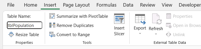
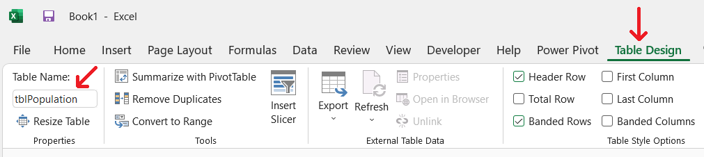
Adding a new table in Excel assigns it a numerical value based on the existing number of tables (Table Name = existing tables + 1), i.e., ‘Table3’ if the Excel file already contains two tables. However, following a custom naming convention is always convenient for referencing tables easily. Users can rename new tables with a prefix such as “tbl” followed by the description of the data set it holds, for example, “tblPopulation.” The tables can be renamed in two ways:

• When selecting the range, click on ‘Insert’ in the menu. You will find the option to change the table name. Change the name as desired relating to the data set selected.

• By clicking on ‘Table Design’ in the menu, you will find the option to rename the table below ‘Home.’

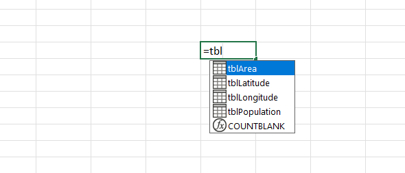
While referencing these tables, we will find that the prefix groups them together, makes it easier to find the required table, and helps us to jump to it directly.

Naming Worksheet

A new workbook usually contains two worksheets: ‘sheet1’ and ‘sheet2’. Imagine a scenario where you are working on an Excel workbook consisting of 50-100 worksheets. It would be quite tricky to determine what type of data is present in ‘Sheet55’ without looking into it. Thus, worksheets should be named based on the inputs/data present in them. For example, ‘Sheet1’ can be renamed ‘Income Statement,’ ‘Sheet2’ can be renamed ‘Balance Sheet,’ and more worksheets can be added to include “Cash Flow Statement” and “Shareholders’ equity” when constructing a model of financial statements. This technique helps create a data flow and gives a general overview of the file.

If multiple worksheets exist with similar names, more descriptions can be added to the sheets to distinguish them from each other. For example, the income statements of different companies on two worksheets can be renamed as ‘Income Statement - TSLA’ and ‘Income Statement - MSFT.’

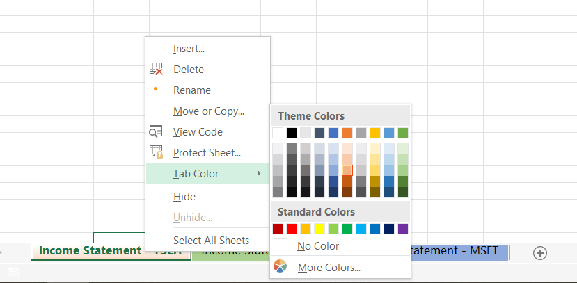
Another tool to help distinguish worksheets with similar names is the ‘tab color’ that adds different colors and gradients to the spreadsheets tab.

It is essential to remember a few key rules while renaming spreadsheets:

• Two worksheets cannot have similar names regardless of the lower or upper case type. For example, saving two worksheets as “income statement” and “Income statement” will give an error to the user. Always use elaborate descriptions to further distinguish the spreadsheets.
• A worksheet name can only consist of a maximum of 31 characters. Excel won’t accept additional characters while renaming sheets.
• Certain characters such as question mark(?), asterisk(*), backward slash(\), forward slash(/), left bracket([), right bracket(]) and colon(:) are debarred while naming spreadsheets.

Naming Charts

Similar to tables, any new charts added are automatically assigned a default value, i.e., ‘Chart 1’ or ‘Chart 2’, based on the existing charts in the workbook. A prefix such as ‘chrt’ or ‘chr’ can be used if your Excel model consists of more than one chart. A chart name should easily communicate the message displayed in the shape of a chart. This helps in the effective transfer of information.

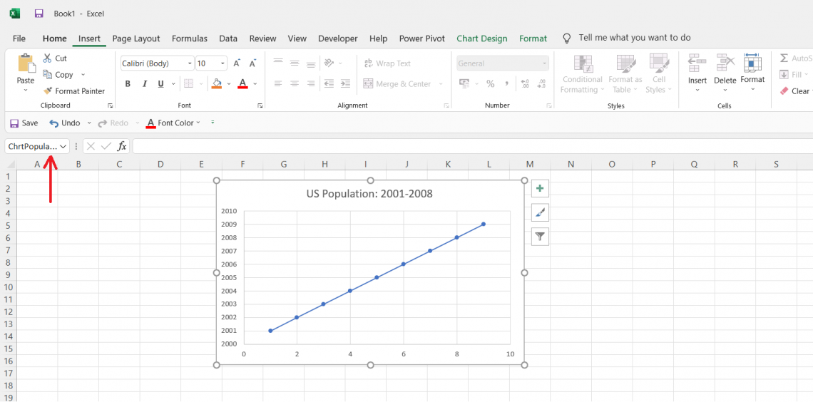
Suppose a chart is to be created based on the increase in the population in the US from 2001-2008 every year, the name of the chart should ideally read ‘chrtPopulation.’ Naming a chart helps to easily use it by referencing it in the Visual Basics for Application (VBA). You can change the name of the charts by following the below procedure:

• Click on the chart, and it will display the name box for the chart below the clipboard.
• Type the name you would like to give for the chart, say ‘chrtPopulation’ in this case, and press Enter.
• The chart name will be saved and can be used as a reference.

Hyperlinks

A hyperlink is a graphic or text button that creates a shortcut to jump to a different spreadsheet in the same Excel file or a web page. A hyperlink to jump onto important sections such as the first page improves the accessibility of the file. The page on which the hyperlink exists is called the source page. For example, if the financial model contains a table of contents, then it will be the source page for all the links to different spreadsheets present in the workbook.

The hyperlinks in a spreadsheet can also be bidirectional, i.e., they can act as the target links in both directions. For example, jumping from the table of content to the income statement and vice versa. The syntax for a hyperlink is :

=HYPERLINK(link_location,[friendly_name])

where,
link_location: This is the file’s path or the location that needs to be opened. It is a compulsorily required field and can also refer to any place in a spreadsheet.
friendly_name: This is an optional field that displays an underlined blue text acting as the jump text for the hyperlink. If the friendly_name argument is omitted, the hyperlink will display the link_location to jump to the desired locations in the spreadsheet.

The two different types of hyperlinks used in Excel are described below.

Cell and file hyperlinks

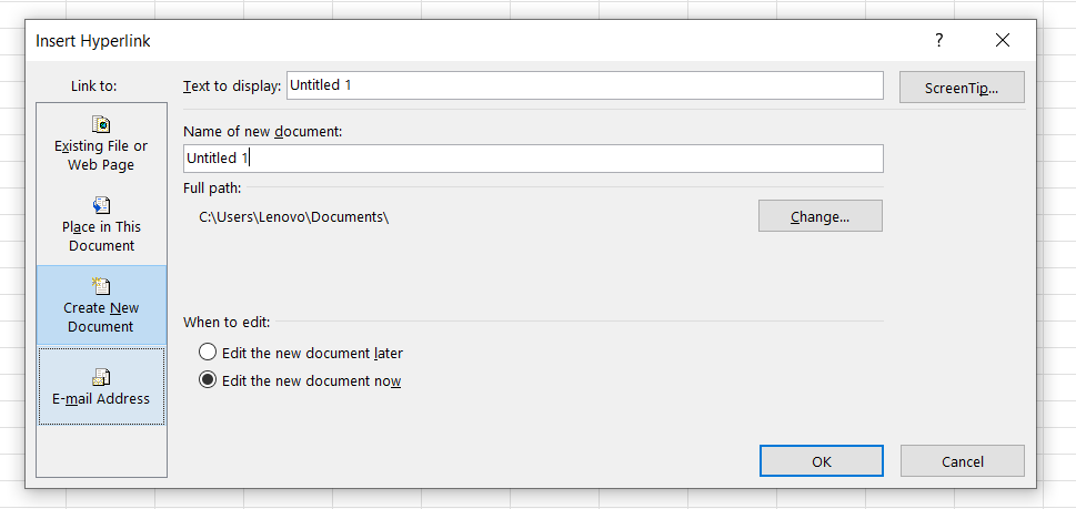
File hyperlinks can be created to access different sections of the Excel file. Since most financial models are long and complex, hyperlinks can help find standard pathways for new users. It can be added to cells or files by pressing Ctrl + K on Windows, which opens the dialog box as shown below.

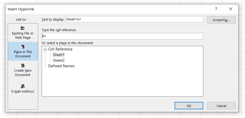
The cell reference above indicates the location to which the cell would jump; in this case, the cell reference is the ‘A’ column, row ‘1’ in Sheet1, i.e., Sheet1!A1. A link that jumps to Sheet1!A1 from Sheet2!Z34 (‘Z’ column, ’34’ row in Sheet2) is an example of cell hyperlinks placed in the same document. Similarly, a new document can also be created, and references can be placed to open the document by clicking on the link created. Here, the text to display represents the link text (also called "anchor text") in the cell for the new hyperlink created.

URL hyperlinks

Hyperlinks can also be set up to directly open the required webpage via the spreadsheet. For example, an external link to download a 10-K can be included in the spreadsheet when working on financial models. However, the external links must be checked thoroughly to avoid unnecessary pop-ups while working on the financial model, which, otherwise ignored, can cause distractions and, ultimately, errors. Therefore, it is good practice to use full URL links for the web pages when linking them to Excel documents.

If the link is missing ‘HTTPS://’ in the web link, MS Excel will automatically assume it and open the correct webpage. For example, if you type www.wallstreetoasis.com in the address bar, it will assume the link to be “https://www.wallstreetoasis.com/” and open the respective page.

A good external link is one that has the same words in the tab of the browser in the same order when clicked on a link. An example illustrating good and bad linking practices is shown below:

1. Bad - This is the Violin Family Wikipedia page.
2. Good - This is the Violin Family Wikipedia page.

Labeling Values

Numerical values tend to look disoriented in the dataset if they lack a readable description. Labels act as a source of information, warnings, or any instructions to improve the financial models’ comprehensibility while working on them.

Consider the two similar data mentioned below for calculating rent roll.

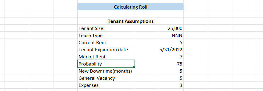
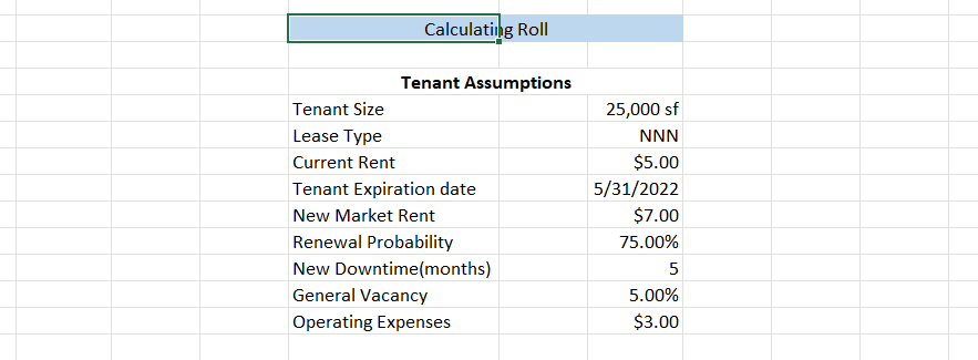
It is easier to understand the second dataset as it properly describes all the underlying units used, while the first seems confusing and is difficult to interpret. Hence, values with proper labels help to reference them conveniently which in turn increases the efficiency of the user of the financial models.

The additional information such as the dollar sign, square feet(area), or the percentage symbol further enhances the narration of the labels. A detailed model always works better than a superficial one.

Cell comments

Cell comments are equivalent to sticky notes that give instructions about the cell. These are indicated by a small red triangle placed at the top right corner of the cell, which displays the comment when the mouse pointer hovers over it. One of the most important objectives for using cell comments is its ability to explain calculations or underlying assumptions in the absence of labeled values.

For example, a cell may have a comment about the error in the formula, which may need to be rectified. In addition, the flexibility of cell comments allows them to resize and change the formatting of text, which makes it an important tool to master while working on Excel models.

Furthermore, cell comments can be of different types.

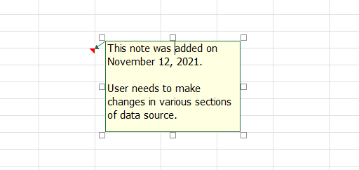
Old comments (‘Notes’ in Microsoft 365)

Notes help store reminders and provide a detailed description of the cell value. They are without “reply” boxes in Microsoft 365, conveying their usage when discussions about the data used are not required. Notes can be inserted by pressing the keyboard shortcut Shift + F2 or clicking Review > Notes > New Notes. The advantage of using notes while working on an Excel file is that they can be used to provide a detailed explanation of the data used in different cells.

Examples of such data include different sources of data used and formulae that need to be corrected, among others.

The only drawback about notes is that all the changes need to be documented with the proper date/time to avoid confusion about their usage.

Actionable comments

Actionable comments have a reply box that allows you to start a conversation with other people working on the same Excel file and take necessary actions about any changes, which can later be marked as resolved. The conversation thread allows accepting or rejecting actions and stores the dialogue with timestamps as they occur while working on the file. To add a comment while working on an Excel model, follow the steps below:

• Right-click on the cell where you want to add a discussion.
• Select New Comment, enter the desired comment, and press post.
• This will initiate a conversation where others can reply to your comment and give necessary recommendations.
• Once the query is resolved, hover over the cell and select more action to click on the “resolve” button.
• If you need to edit your comment, you can hover on the cell, and it will display an Edit option for the comment. In addition, any unnecessary comments can be deleted by right-clicking on the cell and selecting the option called “Delete Comment.”

By using @mention in the comments, you can easily tag someone for the feedback required on the Excel model, as the person mentioned in the comment immediately receives an email along with the link to your comment.

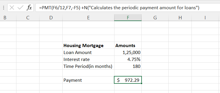
Inside cell comments (Excel function)

The Excel function “N()” is an information function that converts the text inside the parenthesis to zero. The comment inside the parenthesis helps the user understand the logic behind assuming values in complex formulas and their interconnected relationships. It is advisable to be cautious while using this function with numbers as, without quotation marks, it will add the number to the result. The syntax for the N function is

=N(value)

where,
value = text that needs to be converted to zero

The N function can also hold information about the referenced cells or a hardcoded value while working on an Excel model.

Structured references

Structured reference is a distinct method to reference a particular table and its related data (column name) instead of using the cell address in Excel. References can be easily created by simply selecting the table cell and helps to easily locate the table in a large workbook.

One might be tempted to think “What if I change the column’s name that I have already referenced? Do I need to tweak the formula or redo all the work on formulas again?” Absolutely not! When we rename a column, the references also update with the new name. The newly added rows are also added to the existing references with proper calculations as per the formula above the newly entered data set.

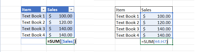
For the above data, the SUM function is used to add the values in H4:H7 using the usual reference, i.e., =SUM(H4:H7), while structured reference is used to get the sum of numbers in the ‘Sales’ column as =SUM([Sales]). So, for example, if the table had a name such as ‘tblBookSales,’ the structured reference formula would read as =SUM(tblBookSales[Sales]).

Structured references - How to create them?

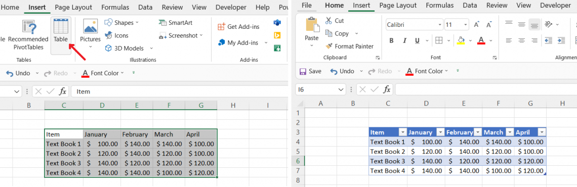
To create structured references, first and foremost, it is essential to select the data and convert it into a table. This can be done using the keyboard shortcut of Ctrl + T or by entering the ‘Insert’ menu and then clicking on ‘Table’ after selecting the data.

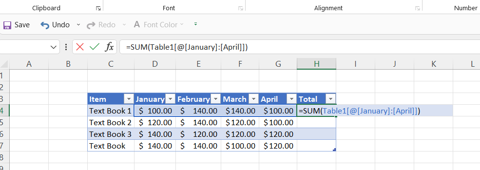
Follow the steps below to create structured references:

• Begin by typing the equality sign(=) similar to typing a formula in a cell.
• Select the cell value that needs to be referenced, and it will automatically capture its heading and create a structured reference.
• Complete the formula by adding a closing parenthesis and pressing Enter. Any formula created inside the table will be automatically filled in the entire column.

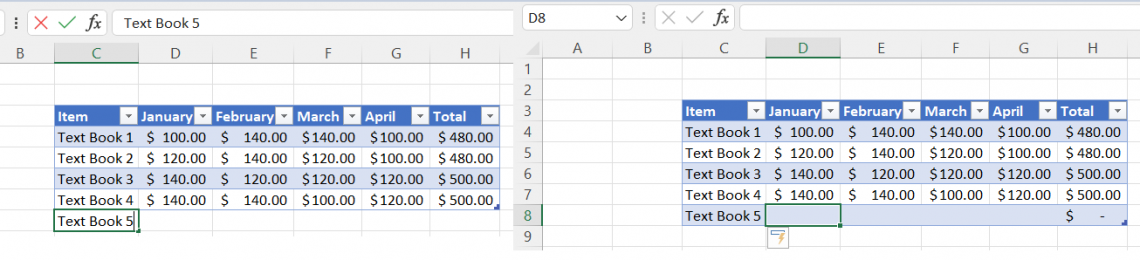
If a new item needs to be added to your data set, just add it at the end and press ‘Tab’ to automatically accommodate it in the table. Even the formula gets filled in automatically, as seen in cell H8.

Data validation

Data validation is one of the most underrated Excel tools. Excel users prefer to learn complicated formulas, functions, and pivot charts and often let data validation go unnoticed due to its simplicity. By ensuring what type of data can be input, the consistency and integrity of the dataset improve significantly.

The Data validation rules can be applied by following the below steps:

• Select a cell range where you want to apply data validation.
• Use the keyboard shortcut Alt + A, V, V or click on the Data tab and then Data Validation to open the dialog box. The ‘Settings’ option will give different alternatives for which data validation can be set up.

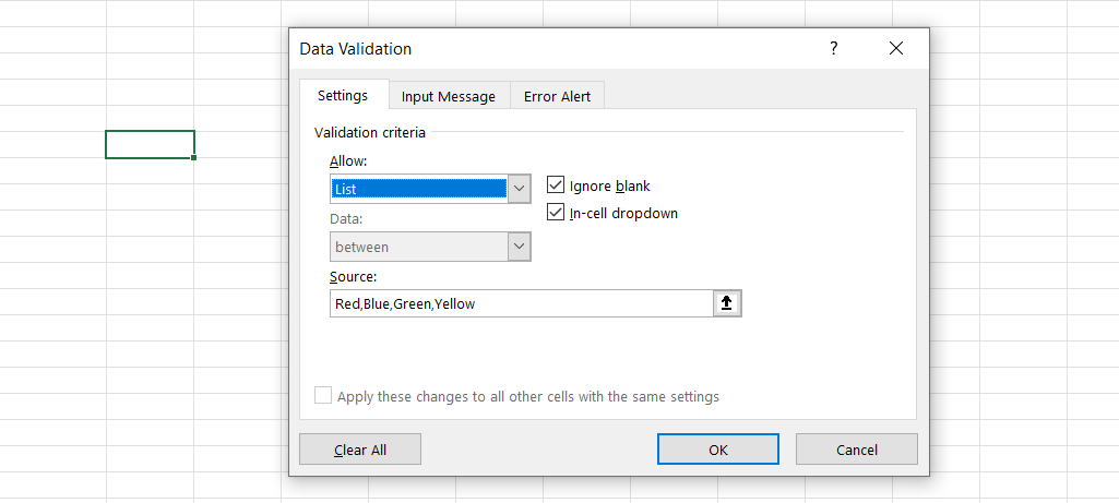
• For this instance, we have allowed a list and manually created a source of four different colors - Red, Blue, Green, and Yellow.
• If we enter a different color value, say ‘White,’ Excel will reject the value by giving an error for it.

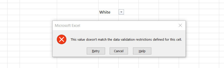
• Only the source colors can be selected, which can be accessed in the dropdown by pressing the keyboard shortcut Alt + Down Arrow key. The list can further create dependent dropdown lists where one item selected will determine what other options appear in the following list.

Hardcoded text

Hardcoded text are the specific values that do not change irrespective of the change in assumptions of the dataset. Therefore, hardcoded values in financial models are used for immutable inputs in formulas.

For example, the actual revenue for the preceding years is usually hardcoded, as it is a historical amount that will not be changed while forecasting the company’s future revenue. Most Wall Street analysts suggest using the color scheme illustrated below for building financial models:

• Blue - For any hardcoded data such as historical values, drivers, etc. This color can be selected by going to More Colors > Custom > Enter the value 255 for Blue.
• Black - For calculations based on the inputs and other references in the same Excel file.
• Green - For calculations and references based on other sheets of the same Excel file.
• Red - For any external links or error warnings.

Find hardcoded text in financial models easily

You needed to make a financial statement model, but you had other work commitments, so you assigned the job to an intern. He has followed all the instructions properly except color-coding the hardcoded text. How can you identify the hard-coded values without going through the entire Excel model individually? Well, let us make it simple for you!

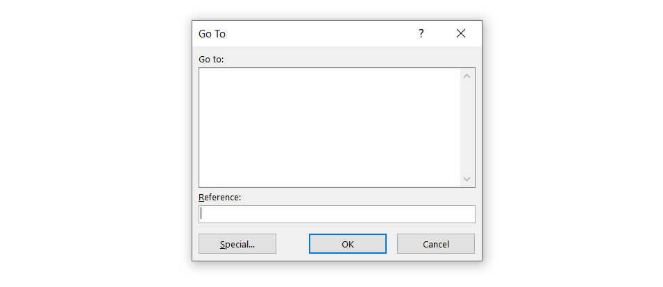
• Press F5 on the keyboard to open a Go To dialog box and click on Special. Notice the underscore(_) below S? If you press Alt + S, it automatically selects the Special option.

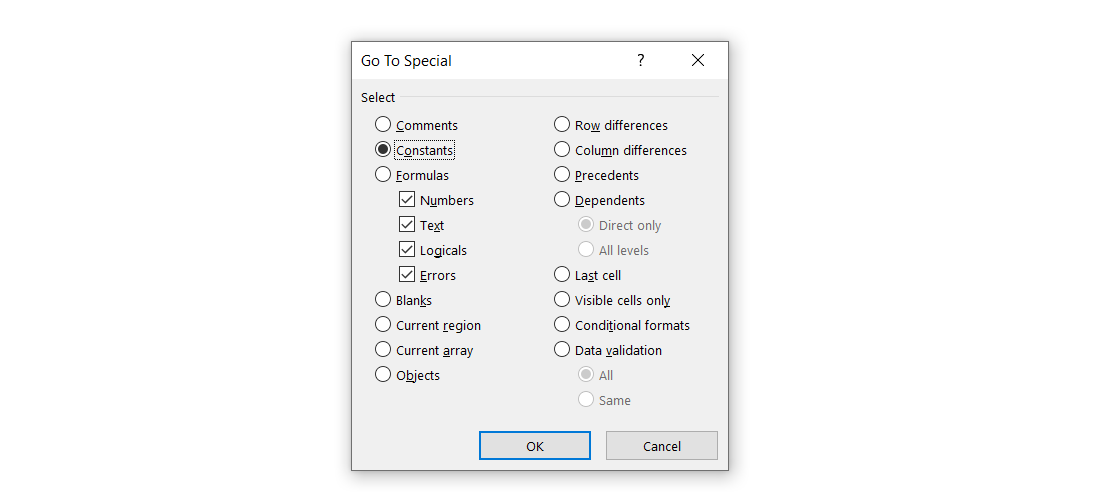
• The succeeding dialog box will display options to select. Since our objective is to highlight the hardcoded values, click on the ‘Constants’ radio button and tick the required checkboxes (Numbers, Text, Logical, Errors). Press Enter to confirm the selection.

Linked dynamic text

A dynamic text is a text that automatically assumes a new value when changes are made in the linked cell. It can be created by simply typing the equal sign (=) in the cell and later clicking on the text for which a dynamic label needs to be created.

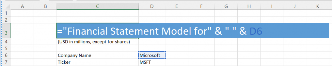
For example, you are assigned to work on the financial modeling of two 10-K’s - Microsoft and Tesla Inc. The cell D6 for the company name can be linked in the header using the concatenate formula or the ‘&,’ whichever is convenient. Here, D6 contains the constant text value Microsoft while cell C3 contains the formula =“Financial Statement Model for”&“ “&D6 resulting in the dynamic text value ‘Financial Statement Model for Microsoft.’ If you intend to include the ticker symbol for the company, just modify the formula to =“Financial Statement Model for”&“ “&D6&D7.

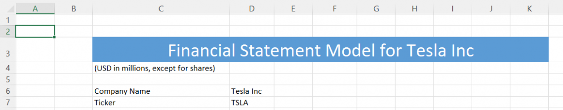
Once the financial model for Microsoft is completed, you can reuse the model for Tesla by typing Tesla Inc in cell D6, and the resulting header will change to ‘Financial Statement Model for Tesla Inc.’ This is one of the simplest examples of linked dynamic text, while more complicated dynamic text can be created using the data validation tool.

Organizing sheets

Unorganized spreadsheets tend to break the flow of information in an Excel model. However, a workbook with organized spreadsheets gives a good overview of the data in the file – such as a master sheet followed by a table of contents, a few worksheets for inputs, a few worksheets for calculations, and final spreadsheets for graphs and results.

If you are working on many sheets, create a table of contents for them. The table with the links to subsequent spreadsheets enables users to easily jump to the desired dataset. Spreadsheets can be organized based on color formatting by left-clicking on the spreadsheet tab and selecting the tab color.

Two differently colored spreadsheets can be easily distinguished if the spreadsheet name is similar. To think differently, it is also a good practice to create a hyperlink in cell =$A$1 to avoid scrolling from dozens of spreadsheets to return the user to the starting spreadsheet (Master Sheet / Table of contents) of the Excel model.

Table of contents

When an Excel file becomes quite large, it becomes difficult to understand the overview of the underlying data. In addition, it is difficult to access different parts of the file without knowing what kind of data might be present in different spreadsheets. The table of contents helps to solve this problem by linking all the corresponding spreadsheets from a single master sheet.

The most basic method to create a table of contents is to manually create it:

• Insert a new spreadsheet by using the keyboard shortcut of Shift + Alt + F1 and rename it by double-clicking on it to ‘Content.’
• Type the sheet name and give a short description if the spreadsheet holds multiple data sets.
• Using a keyboard shortcut of Ctrl + K, a dialog box will open to hyperlink the sheet name to the Excel sheet in the spreadsheets tab. When jumping to different spreadsheets, it is best to reference the first cell, i.e., A1, on the sheet. Unless there is a special requirement, the value for cell reference can be kept as ‘A1’.
• Click on a worksheet and repeat the steps until each worksheet is linked to the table of contents.

Instruction sheet (if necessary)

An instruction sheet helps replicate the task easily if re-run by the third person. Sometimes, situations may arise where your colleague might have to work on the financial models prepared by you and might not be aware of the assumptions or different references in the Excel file. Hence, it is of utmost importance to have a separate spreadsheet imparting them with knowledge about the model.

These instructions should be detailed with different parameters such as font, font size, alignments, formula, references, etc. The efforts made in making the instruction sheet might even help our future self if we use it again after not working on the file for a long time.

Most VBA models also have an ‘instruction sheet’ with a protocol that needs to be followed to complete mundane tasks easily.

Why document?

Documentation indicates significant changes made in the history of the spreadsheet. It may include different parameters such as the overview of the model, how to use the spreadsheet, what output is to be expected based on the calculations made, the required input data and its format, and version details. The documentation of Excel models preserves the standard operating procedures for the successors handling them, helping them make decisions based on the different output scenarios of the financial models.

For others

Many different analysts might refer to the Excel model prepared by you during your tenure at the organization. Even after you leave the organization, a source must exist that could be referred to to understand the workings of the Excel model. After final validation and approvals, the process flow and the comments in these documents will save a lot of time for your successors and senior management.

For example, suppose you are working on a different project. Your successor did not attend the meetings where you discussed all the intricate relationships between various elements of your Excel model. Then, he might find it difficult to understand it without proper reference documents. Documentation also needs to replicate the thinking process behind the model and the knowledge utilized. A detailed document just ticks all the boxes.

For yourself

Since we developed the financial models, it might be expected of us to remember all the logic and sources of information used in Excel models. However, in reality, this is not possible. It is absurd to believe that a person will remember the exact details that clients and higher management have requested to be included in the financial models over time.

Most of the complicated Excel models are built via information exchanges through client calls and management meetings. Further, you may be required to work on different Excel models during your tenure at the organization. Hence, only with proper documentation on using the Excel model can we help it stay relevant months later.

More on Excel

To continue your journey towards becoming an Excel wizard, check out these additional helpful WSO resources.

• Excel keyboard shortcuts for Windows and Mac
• Advanced Excel formulas you must know
• Best Excel courses
• Developer tab
• INDEX MATCH formula