FV Function Excel

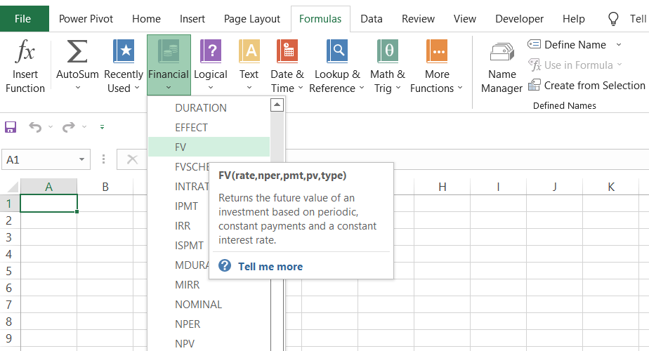
What Is The Excel FV Function?

The FV function in Excel calculates the future value of an investment based on predefined inputs.

By employing the present value of the investment, the holding period, and the expected rate of return in the formula, you can return the future value to compare two different investment alternatives.

In this article, you will see how to use the FV function in Excel and its application in real-life scenarios. FV, an acronym for future value, is a financial function that returns the value of an investment in X period (s) in the future.

For example, if you invested $1000 today, which yields a return of 5.05%, with a maturity period of two years, the future value of the investment will be $1,106.04. Here, the growth rate for our investment is 5.05%, which yields $106.04.

As an investor, it is essential to know what the asset's value will be in the future if you choose to invest today. We are well acquainted with the time value of money, which states that a dollar today is worth more than a dollar in the future.

If you forgo that money and invest it, let’s say you need some incentive counteracting the opportunity cost to secure your retirement. This is because that money could have otherwise funded, for example, a new car or a vacation in the Bahamas.

The inclusion of incentives in the form of returns makes it essential to calculate the future value of the investment.

Inflation will still decay the value of your asset. On the bright side, you could potentially secure your child’s education and other financial needs based on the future value estimation.

Calculations to determine FV Function

You can use two formulas to calculate the future value, depending on the type of interest earned - simple interest or compound interest.

The calculations for an investment earning a simple interest rate are relatively easy since the interest does not compound over time. The formula to calculate a future value for a simple-interest investing is:

FV = PV (1 + RT)

Where,

• PV = present value of the investment
• R = rate of return on investment
• T = time period

On the other hand, when an investment generates interest on the principal amount and, in turn, the interest balance further generates interest on itself, the investment is said to be compounding.

The formula to calculate the future value for a compound-interest earning investment is:

FV = PV ( 1 + R )^T

Where,

• PV = present value of the investment
• R = rate of return on investment
• T = time period

The syntax for the FV function in Excel

The syntax for the FV function is:

= FV(rate, per, pmt, [pv], [type]

where,

• rate = (required) The interest rate for the period. This can vary depending on whether the interest rate is annual, monthly, etc.
• per = (required) the total number of payments for the period
• pmt = (optional) The payment for each period is expressed as a negative number. The PV argument must be included if you omit the pmt argument.
• PV = (optional) This represents the present value of the investment. It is expressed as a negative number in the formula and, if omitted, pmt must be included, or the initial investment becomes zero.
• Type = (optional) Defines the time when the payments are made for each period. If the value is 0 (default), the costs are made at the end of the period. If the value is 1, they are made at the beginning of the period.

The rate and the number of payments must be in a consistent format. For example, if you use an annual rate, then costs must be annualized.

If the payments are made monthly, an annual rate would be divided by 12 (for example, 8%/12). 

Examples of the FV function in Excel

The FV function becomes easy to use once you understand the arguments you need to input into the formula. We will see different situations where you can use the FV function by tweaking the recipe.

1. FV for a lump sum + periodic payments

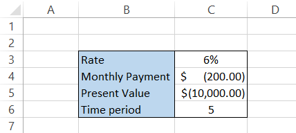
Assume that you have $10,000 in your savings account, earning compounded interest annually at 6%. Let’s say that you decide to make $200 monthly contributions to the savings account for five years.

By summarizing the data in Excel, it will look as illustrated below:

Since we make monthly payments, we also need to represent the rate and period in terms of months.

Thus, the formula that you will use to find the future value of the investment after five years will be =FV(C3/12, C6*12, C4, C5,1), giving you $27,512.28

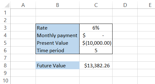
2. FV for a lump sum

We have assumed that all the monthly payments are made at the beginning of the month, considering salaried individuals. Let’s say no monthly payments will be made, and the interest will compound annually on the principal amount of $10,000. What would its future value be? Here, we will exclude the pmt argument so that the formula becomes =FV(C3, C6, C5,1). The yearly breakdown for the interest earned on the principal amount is below:

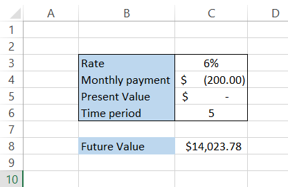
3. FV for monthly payments

Let’s assume you intend to only make monthly payments of $200, with no initial lump sum. You’ll do this for the next five years and earn 6% annually. The future value of the investment will be calculated using the formula:

=FV(C3/12,C6*12,C4,,1)

This will give the result illustrated below:

As opposed to the lump sum amount, the compounded interest earned for the same period equals $2023.78.

Ensure that the outflows, such as monthly payments or deposits made for investment, are represented as negative numbers in the spreadsheet. In the formula, you can also use a negative sign(-) before the PMT and PV argument.

Practical Example of the FV Function in Excel

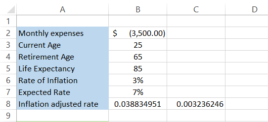
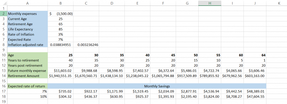
Let's say you are 25 years old and have decided to start saving for retirement. You currently spend $3,500 monthly. The mutual fund you choose to invest in has a return rate of 7%.

Assuming that you would retire at the age of 65 and a life expectancy of 85 years old, the data looks as illustrated below:

First, you are investing because inflation depreciates the value of money over time. By supporting the money, you potentially stop depreciation and build wealth.

For our data, the rate of inflation is 3%. We have another factor in our inputs - the inflation-adjusted rate. The inflation-adjusted rate considers the effect of inflation on the investment and shows an inflation-free return.

Here, we have used the formula =(1.07/1.03)-1 in cell B8 to calculate the inflation-adjusted rate. For convenience, we have calculated the monthly inflation-adjusted rate in cell C8 by dividing B8 by 12.

The next part of the model is finding the final value of the retirement fund.

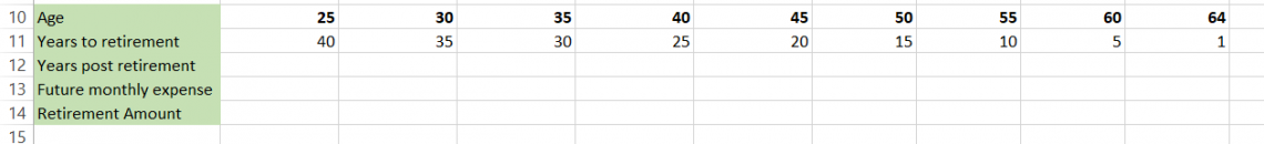
This section of the Excel model will show you what the retirement amount will be based on your age. So, if you start saving for retirement at 25, you have 40 years to save, while if you start at 30, you will have 35 years to save for retirement.

The “Years post-retirement” row is found by simply subtracting retirement age from life expectancy, i.e., 85-65 = 20. This means you need a retirement account that will be enough to suffice for 20 years.

You currently have monthly expenses of $3,500, but you will also need to forecast what your monthly payments will be in the future. Inflation leads to an increase in the overall cost of living.

Per a study by M. Shahbandeh, a gallon of milk cost around $3.74 in the US in the year 2021. However, the same gallon of milk costs around $2.52 in 1995.

Thus, an increase in prices due to inflation ultimately means you will pay higher monthly expenses each year.

To find the future value of monthly expenses, we will use the formula =FV($B$6/12, B11*12, $B$2,0) in cell B13, which will give the monthly expenditures after 40 years at the age of 65 as:

You should interpret this table in reverse order. This means that after 40 years, your monthly expenses will be $11,603.02, while the costs after a year, i.e., at the age of 26, will be $3,606.46. However, this doesn't say how much we should save.

We will use another function - the present value to find the retirement corpus. The PV function finds the current value of the investment based on its future value/monthly payment. The formula that you will use is =PV($C$8, B12*12,-B13,,1), which will give you the result as:

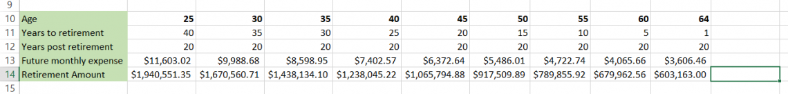
So, for a life of 20 years post-retirement, with monthly expenses of $11,603.02 at the age of 65, you will require a retirement account of $1,940,551.35.

So, how much will you have to deposit monthly to achieve this goal?

To calculate the monthly payments you need to make from the age of 25, you will use the PMT function, creating the formula =PMT($A$17/12, B11*12,0,-B14,1), which will give you the payments that you need to make in the mutual fund to yield the required retirement account at age 65.

This will give you the result as illustrated below:

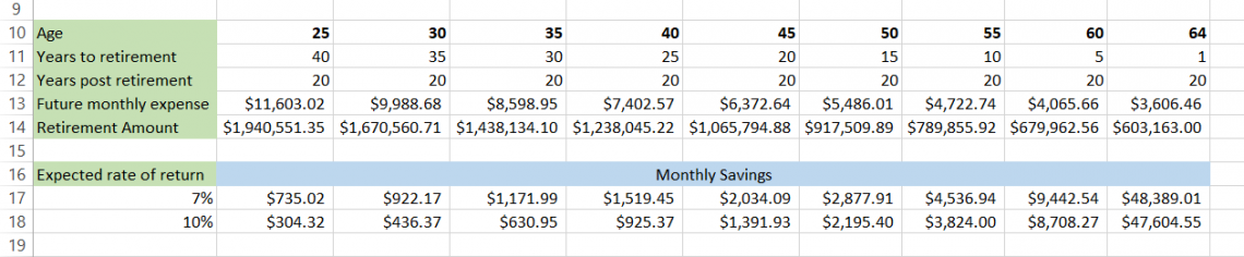
If you invest in a fund that gives 7% returns, you must invest $735.02 monthly until age 65. If you find a better mutual fund option that gives you 10% returns, the monthly payment becomes $304.32.

Let’s say you decide to start investing at the age of 40. Now, you must make monthly payments of $1,519.45 with a 7% rate of return and $925.37 with a 10% rate of return.

Now, you can tweak the numbers, find what works best for you, and plan your retirement goals. The entire Excel model looks as illustrated below:

As we needed to find the monthly expenditure, we expressed the inflation-adjusted rate as a monthly rate instead of an annual one.

To conclude, using the FV function, you can find the future value of an investment and make informed decisions depending on what investment has the most outstanding returns compared to the alternatives.

Researched and Authored by Akash Bagul | Linkedin

Reviewed and edited by James Fazeli-Sinaki | LinkedIn

Free Resources

To continue learning and advancing your career, check out these additional helpful WSO resources:

• PEARSON Function
• PI Function
• SEARCH Function
• SQRT Function
• SUBTOTAL Function