INDEX Function
Returns the cell reference for a value based on the row and column number specified, ultimately returning the value from an array


What Is the INDEX Function?
The INDEX function in Excel returns the cell reference for a value based on the row and column number specified, ultimately returning the value from an array.
Assume that you are on a road trip traveling to Kansas City. To your amazement, you check on the map and find two places named ‘Kansas City’. One is in Kansas state, while the other is in Missouri.
Unsure about where to head, you text your friend, who sends you the coordinates for the city as 39.0997 degrees N, 94.5786 degrees W. Next, you check Google Maps and find it to be Kansas City in, Missouri.
What happened here?
The coordinates act as the row and the column number, whereas the world map serves as the array from which the coordinates pinpoint the specific position.
The INDEX function works on the same principle and even works as a lookup function when combined with the MATCH function.
In this article, we will see what an INDEX function is, its syntax, and a couple of examples to understand it better.
- INDEX is a powerful Excel function used for retrieving values from an array based on specified row and column numbers.
- Understanding the syntax is crucial. The function structure consists of the array or reference, row number, and optional column number or area number for more complex arrays.
- INDEX function aids in various scenarios like left lookups, two-way lookups, dynamic range calculations, and extracting specific data points from arrays.
- Combining INDEX with MATCH expands its utility, offering advanced lookup capabilities and flexibility, especially for large datasets.
- Beyond lookups, INDEX facilitates tasks like retrieving all values in a row or column, obtaining the last value in a range, and creating dynamic ranges for calculations, enhancing efficiency in Excel data management.
Understanding the INDEX function
The INDEX is categorized as a Lookup and Reference function that returns the value in a given array based on column and row number.
For example, suppose that you have stock price data as illustrated below:
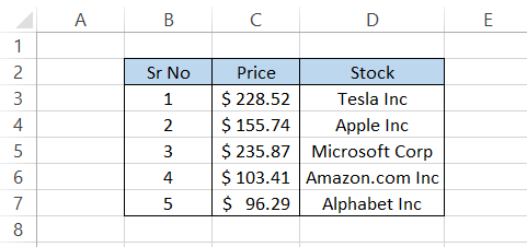
If we wanted to find the price of Microsoft Corp price visually, what we usually do is find the row and column in which the value intersects in the given table.
As you can see, the Microsoft Corp stock price of $235.87 intersects at column C and row 5 or cell C5.
Thus we get the stock price of $235.87 when we reference the range B2:D7 as our array while inputting the row and column as 5 and C, respectively.
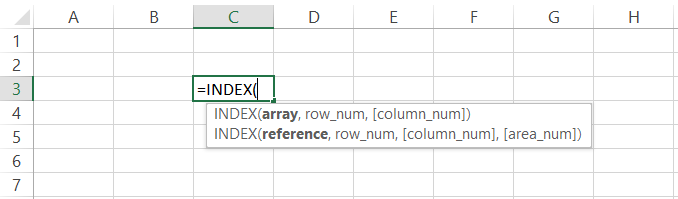
The syntax for the function is:
=INDEX(array, row_num, [column_num])
where,
- array - (required) range of cells from which the function returns the required value. The subsequent row_num and column_num are optional if the array consists of a single row and column.
- row_num - (required) the row number from which the function extracts the value. The column_num argument is required if the row_num is skipped.
- column_num - (optional) the column from which the function extracts the value. column_num can be skipped if the required value is based only on the row_num argument.
An alternate syntax exists for the function, called the reference format for the INDEX function. The syntax is:
=INDEX(reference, row_num, [column_num], [area_num])
where,
- reference - (required) the reference to cells or multiple ranges of cells. Whenever you reference multiple ranges of cells, each range should be separated by a comma (for example, A3:A7,E3:E7,Z3:Z7…)
- row_num - (required) the row number from which the function extracts the value. The column_num argument is required if the row_num is skipped.
- column_num - (optional) the column from which the function extracts the value. column_num can be skipped if the required argument is based only on the row_num argument.
- area_num - (optional) this argument allows the user to determine what range to use for returning the value from multiple referenced ranges.
For example, if you have ranges as A3:A7, E3:E7, and Z3:Z7 and assign the number 3 for area_num, then the function uses range Z3:Z7 for retrieving the value. However, if the area_num is skipped, then the default value of 1 correlating to the first range is assumed.
How to use the INDEX Function in Excel?
Since the function comprises only three arguments, it is relatively easy to use. We spoke in depth about the syntax, so we will head over to how to use the function as a worksheet formula.
Suppose that you have the data as illustrated below:
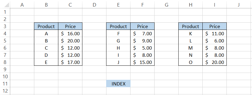
To use INDEX in the array format, we will use the formula =INDEX(B3:I8,5,4), which gives us the result as product ID - I.
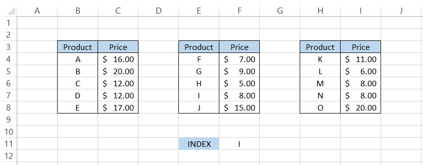
You must be wondering, since we input row_num as 5 and column_num as 4, shouldn’t the extracted value be from cell D5 by traditional cell count?
As you might see in our reference argument, we have input the range as B3:I8, which changes everything for us.
Now, whatever intersects at row and column are 5 and 4 in our selected array, the corresponding cell value is returned as a result, i.e., cell F11.
If you want to use the function in a reference format, the formula will be =INDEX((B4:C8,E4:F8,H4:I8),4,1,2) which also gives us the product ID - I.
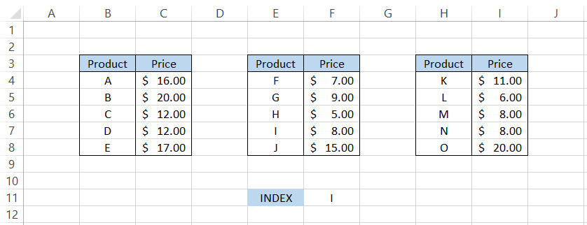
Here, we input multiple ranges, type in the row and column number, and finally select the range we need to extract the value. For example, we set the second range E4:F8 by inputting the area_num as 2.
INDEX Function Examples
Using the function by itself might have limited application. However, if you use the function with the MATCH, then it takes the lookup functionality to a whole different level.
You will only sometimes count the row and column numbers from the referenced array and try to return a particular value.
Counting rows and columns would be especially tedious when working with large data sets. This is where you can use the combination of the INDEX MATCH function, which works even better than VLOOKUP or HLOOKUP.
1. Example #1 - Left lookup
When using VLOOKUP and HLOOKUP, you cannot leverage the power of the function to make left-side lookups.
You can use the INDEX MATCH, bypassing this limitation and returning the error to the user without manipulating the data.
Suppose that you have the data as illustrated below:
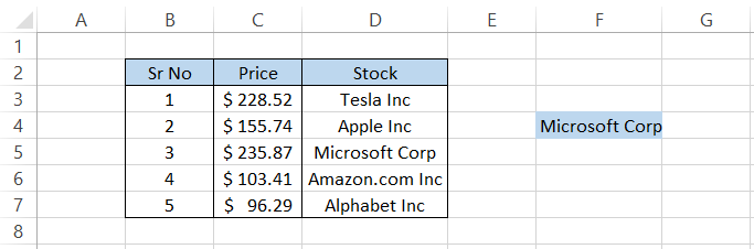
In this table, the stock name lies on the right side while the prices are on the left side, meaning we might need to do a left lookup to avoid data manipulation.
We will use the formula =INDEX(C3:C7,MATCH(F4,D3:D7,0)) in cell G4, which gives the price of Microsoft Corp as $235.87.

What happened behind the scenes is that:
- The MATCH function finds our text string's first 'match'.
- The INDEX function then finds the cell corresponding to that of the 'matched' cell.
- The MATCH function found the result in cell D5, upon which the INDEX function returned the result as C5 since we had referenced the range C3:C7 in our formula.
2. Example #2 - Two-way lookup
Remember, we have the column_num and the row_num argument in our INDEX function. However, in the earlier example, we had only used one MATCH function in place of the row_num argument.
In this example, we will see how you can use two MATCH functions for a two-way lookup scenario.
Assume that you have the data as illustrated below:
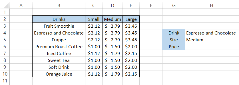
To make use of the two-way lookup, we will use the formula =INDEX(C3:E10,MATCH(H4,B3:B10,0),MATCH(H5,C2:E2,0)), which gives the result as $2.89.
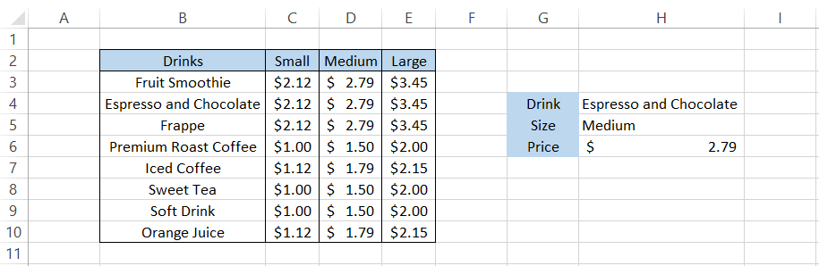
Three things happened behind the scenes:
- The first MATCH function finds the position of 'Espresso and Chocolate' in range B3:B10 and gives the result as row 5 (since we have substituted the function in place of the row_num argument.
- The second match function finds the position of 'Medium' size in the range C2:E2 and gives the result D column.
- Finally, the INDEX function finds the intersection of the rows and columns, giving the final price of medium-sized Espresso and chocolate $2.89.
The pros of using the INDEX function and MATCH far outweigh using either of the two functions separately.
Other Uses of the INDEX Function
Although INDEX MATCH is one of the most important tools in Excel, the function also has a vast range of capabilities.
It can be used with the conditional formatting tool or as a worksheet formula to return a particular value in the given cell.
1. Calculating the SUM of top 'n' items in a given list.
Although the function returns the value, as a result, the INDEX originally finds the cell reference for the given value.
This opens up the possibility of using the function with other functions, such as SUM, AVERAGE, MIN, MAX, etc., to create dynamic ranges.
One of the applications of those dynamic ranges is finding the SUM of top 'n' items in a given dataset. For example, suppose that you have the data as illustrated below:
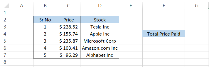
We want to determine the total price paid for the first three stocks. This means we will use the SUM function along with the star of our article.
The formula will be =SUM(C3:INDEX(C3:C7,3)), giving the total price paid as $620.13.
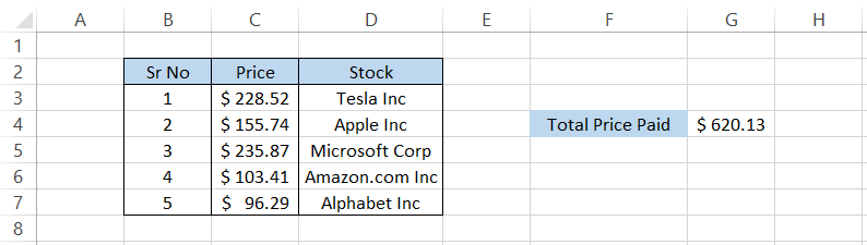
Do you see the numerical value 3 in our formula? That signifies the number of cells from the top for which the function will take the SUM. So, for example, when you add $228.52 + $155.74 + $235.87, you will get the same result, i.e., $620.13.
2. Getting all the values
Another situation where you can use the function is to retrieve all the values in a column or a row in Excel.
The only criteria you need to remember is that if you are getting the values in a row, you need to omit the column_num argument or input zero and vice versa.
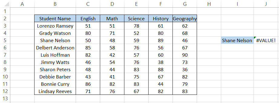
Assume that you have the student test scores as illustrated below:
Here, we will use the combination of the INDEX MATCH function using the formula =INDEX(C3:G12,MATCH(I5,B3:B12,0),0), which surprisingly gives us the #VALUE! Error.
You would ask, "What next?"
The next step is crucial: you edit cell J5 using the F2 key and then press the F9 to make manual calculations while the cell is in edit mode.
You will get the result:
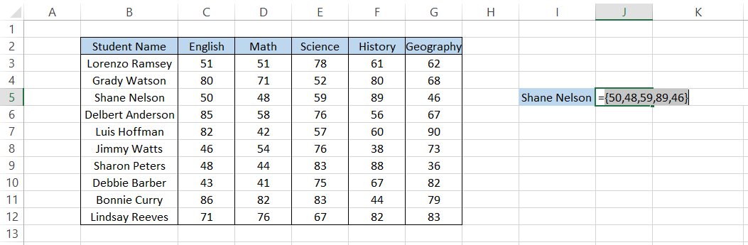
You can copy this array of numbers using the Ctrl + C and then Paste Special them as 'values' in a different cell. This trick can be quite handy to get all the values across a row or column.
3. Getting the last value in the range
We saw how you could get all the values in a row or column in the previous example.
What if we wanted a value at the end of the range without scrolling through thousands of rows of data?
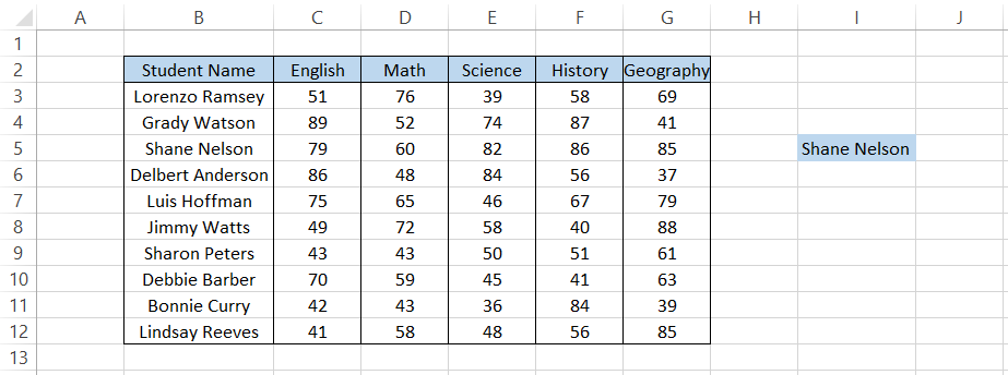
In this case, we can use the INDEX function and the COUNTA. For example, suppose that you have the data as illustrated below:
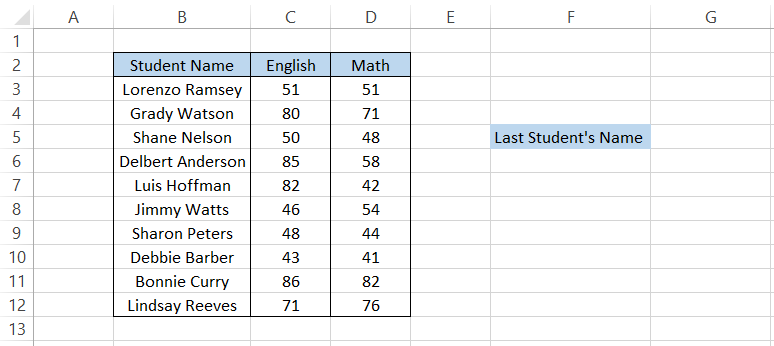
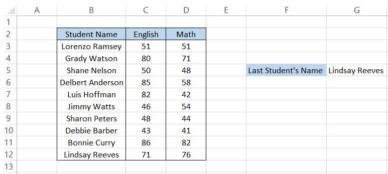
To get the last student's name, we will use the formula =INDEX(B3:B12,COUNTA(B3:B12)), which gives the result as Lindsay Reeves.
The only downside to the formula is that it will not work if there are empty cells in the referenced range. This is because the COUNTA function plays an integral role in this formula, which counts all the cells with any information.
When an empty cell is encountered, the counter resets to zero; thus, we get zero as our result. On the other hand, if all the cells in the referenced range have any value, the formula finds the last cell and returns the same result in the spreadsheet.

Free Resources
To continue learning and advancing your career, check out these additional helpful WSO resources:


or Want to Sign up with your social account?