HLOOKUP Function
A function that helps search for a value in the top row of a table or an array and returns the value in the same column from a specified row below the table.


What is the HLOOKUP Function?
The HLOOKUP function is an acronym for ‘Horizontal lookup’, which helps to find and return a value from a horizontal table as our source. Similar to the VLOOKUP, it searches for the lookup value in the first row of the table and returns another value based on the match it finds in the adjoining rows.
It is useful when the lookup value is located at the top of the table, and you need to retrieve another value that is located a few rows below.
The HLOOKUP function will let you retrieve data using the lookup value in a horizontally organized table. For example, assume that we have the prices for the medium-sized Mccafe drinks in a horizontal table as below:
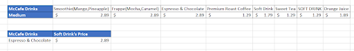
If we intend to find the price for ‘Espresso and Chocolate,’ we can use the HLOOKUP function where our lookup value will be in cell B7, the range will be the table, and the value returned will be $2.89.
- Values are placed across the columns in horizontally organized data, which is the format in which HLOOKUP is intended to operate.
- Give the table_array argument the appropriate range of cells that contain the data you wish to search through. The lookup values should be in the top row of this range.
- Specify the row_index_num parameter accurately to indicate which row below the top row contains the data you want to retrieve.
- The choice of whether HLOOKUP should produce an exact match or an approximate match is made by the optional [range_lookup] argument.
Syntax for HLOOKUP
The HLOOKUP function consists of four different arguments:
=HLOOKUP(lookup_value, table_array, row_index_num, [range_lookup])
where,
- lookup_value = the value to look for in the beginning of the table, i.e., first-row value
- table_array = the table from which the value is to be retrieved
- row_index_num = this parameter intends to retrieve value from our expected row
- range_lookup = optional parameter [TRUE] = gives an approximate match if the exact match is not found, [FALSE] = gives the exact match or will return an error if the exact match is not found.
The simpler version of the HLOOKUP can be stated as:
=HLOOKUP(The value that you are looking up, the range where you are looking for the value, the row number for the selected range in which the value exists, Approximate(TRUE) or Exact Match(FALSE))
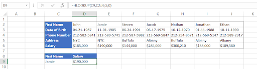
For example, if we need to find how much Jamie earns every year, we will use the HLOOKUP function, which would return the value as $190,000 since our row_index_num is 5.
How to use the HLOOKUP Function in Excel?
Using the horizontal lookup function is not rocket science.
First, you must set up the dataset on which you intend to perform the horizontal lookup. The HLOOKUP function will then search the top row in the table for a value that matches your search criteria, and return a corresponding value from the same column.
STEP 1: Arrange your data from top to bottom
HLOOKUP can only find values when the lookup_value are located in the first row of the table. It means that if your look_up value is at the end or in between the table, it will fail to retrieve the value and throw out an error.
Arrange the data in such a way that the look_up value is in the first row at the top and all the corresponding information that you need to retrieve is below the look_up values to avoid getting the #N/A error.
STEP 2: Identify the look_up value
Lookup_value defines what the user is looking for, which could be names, numbers, or even dates. For example, in this case, our lookup_values are in row 2 starting from column C, represented by the header ‘Year.’
STEP 3: Define the table_array
HLOOKUP needs to know where to find the lookup_value and, if found, what value to return from the selected range or the table. This condition is fulfilled by defining the table_array in our function.
You can select the table_array from the same or two different spreadsheets as well as entirely different workbooks. For example, our table_array in this dataset is range C2:J5.
STEP 4: Row_Index_Num
The third argument in our function is defined by numbers. The row_index_num acts as a constraint and specifies the row from which we want to retrieve the value. Excel is smart, but it is not that smart to determine what row to obtain the value from; hence we need to specify the row_index_num in the function.
Our table_array has four rows, and row_index_num can be either 1,2,3,4 (Using the row_index_num as 1 does not make sense and does not provide much value to the users unless it's a reconciliation task).
Note
You will receive a #VALUE! Error if the row_index_num is less than 1.
STEP 5: Choose between Exact and Approximate value
This is an optional yet the most important parameter of the horizontal lookup function. It commands Excel to find either an exact or approximate match for the lookup_value. The default value is always TRUE(1) if you don't mention or skip the argument.
However, by using the FALSE(0), you can get an exact match for the data and avoid all the wrong results while looking for data.
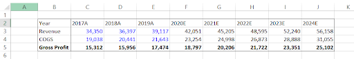
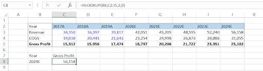
For example, let's say we want to find the gross profit for the expected year 2022 from our three-statement financial model made by Nike. To do this, type the formula
=HLOOKUP(B8,C2:J5,4,0)
We have referenced cell B8 so that we can dynamically change the value to different years, and it will automatically display the gross profit for the referenced year.
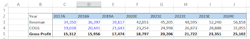
In this case, the gross profit in the year 2022 is $21,722. Similarly, if we want to find the estimated revenue in the year 2024, we just need to change the row_index_num to the row from which we expect our value.
Here, we change our row_index_num from 4 to 2 by changing our formula to =HLOOKUP(B8, C2:J5, 2, 0), which will give us the estimated revenue in 2024 as $56,158.
Exact Value in HLOOKUP
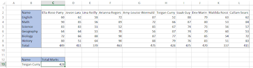
Based on the range_lookup argument, HLOOKUP can perform two types of lookup: FALSE for an exact match and TRUE for an approximate match. By default, Excel uses the TRUE parameter in the formula. Assume that you need to find exactly what the total marks scored by ‘Teigan Curry’ in his examination.
The dataset looks as follows:
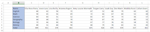
For this, you can use the formula =HLOOKUP(B13, C2:L9, 8, FALSE), which uses the range_lookup argument as FALSE to retrieve the exact value. If you had used TRUE as the optional argument, the result would have been 411, which is not even closely related to the total marks scored by Teigan.
Approximate Value in HLOOKUP
The approximate argument method returns the next largest value, which is smaller than our lookup_value.
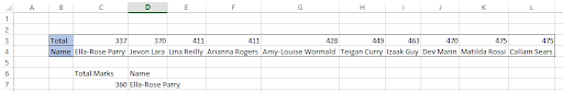
For example, let's say you know someone has scored total marks around 340-360 or below. You need to know the name of the student to assign him extra lectures which are scheduled for the end of the month. The dataset looks as follows:
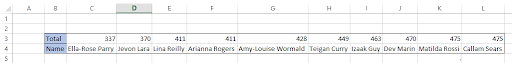
Here, you can use the formula =HLOOKUP(C7,C3:L4,2,TRUE) with the lookup_range argument as TRUE. Note that our look_up value is 360 (upper limit), and the HLOOKUP will return the student's name that has scored marks nearest but lower than our lookup value.
We get the result as Ella-Rose Parry who has scored a total of 337 marks in the exam.
Note
You must always arrange your look_up values in ascending order; otherwise, the formula will give you the wrong result.
HLOOKUP Function Uses
HLOOKUP is commonly used in two scenarios:
- When you're looking for a value in a horizontal table, and you know what row the value exists in. For example, suppose you have a list of employees and need to know the address present in row 5. By specifying the row number, you can retrieve the address for the employees.
- To check whether a particular value exists in our horizontal table. For example, assume that a Burger King employee checks the order summary based on the order no. for the customers as the lookup_value, and if the result gives an #N/A error, it means that the order for the customer does not exist in the database.
In both cases, the “‘lookup value’ specifically helps to find or return the value we want.
HLOOKUP in financial modeling and financial analysis
Horizontal lookups work great in retrieving the data in financial models or making sensitivity models since they are oriented in a horizontal perspective.
Suppose you have made assumptions tables about the revenue growth driver in your financial model. So if your current annual revenue is $42,051 million and today's date is December 15th, 2021, Excel pulls up an expected value for December 15th, 2022, of $45,205 million based on the revenue growth driver using the HLOOKUP function.
You don't have to calculate this yourself!
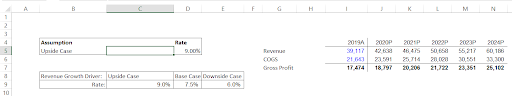
In the example above, we use the formula =M5*(1+HLOOKUP($B$5,$C$8:$E$9,2,FALSE)) to pull in the data from revenue growth driver assumptions in cells C8:E9.
Simply by changing the value in cell B5 to either the upside case or the downside case, our financial model will reflect the revenue based on a 9% rate for the upside case or a 6% rate for the downside case.

Advantages of HLOOKUP
Some of the advantages are:
- Dual matching mode - The two modes of matching help the user to find either an approximate match or an exact match by specifying the optional parameter either as TRUE or FALSE, respectively.
- Comparatively easier to use - The function consists of four arguments, out of which one is optional (yet important). No tricky conditions or nested formulas, just select the lookup value, reference the table and enter the number from the row from which you expect the result. It's that simple!
- Saves time - Though most of the time, horizontal tables might not consist of a lot of data/rows, you can still save a lot of time that can be spent in searching for the value manually.
Limitations of HLOOKUP
The limitations include:
- No bottom-to-top lookups - This means that your data must be oriented from top to bottom only with your look_up value at the first row or the top row. The function will not work if there are values at the top of your lookup_value and they are referenced as table_array in the function.
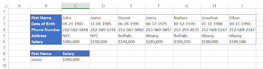
- Matches first value in case of duplicates - Suppose you need to find the salary for ‘Jamie,’ i.e., cell F2 from your employee database, who lives in Albany. There is another Jamie who lives in New York City.
By using the first name as our look_up value, enter the formula =HLOOKUP(B9,C2:I6,5,0) in C9. This gives us the value of $190,000.
In case you need to, check out our article on VLOOKUP here, which explains how to deal with duplicates.
However, on closer inspection, we check that the results retrieved are actually wrong.
Even after referencing the correct first name, the formula matches the result for the first value, i.e., for cell D2. This makes it quite a hassle in case there are duplicate values in our lookup value row, which is usually in the case of date/name or a year.
- Static references - If you insert or delete rows in your table_array, you might get #REF! error as a result of references becoming invalid. In such cases, you need to edit the formula again to make valid references again.
- Slower calculations - Exact match mode iterates through every single cell of our referenced table_array. So, if your table consists of hundreds or thousands of rows of data, it can cause Excel to slow down, affecting your work efficiency.
- It is not case sensitive - When you want to retrieve a value, HLOOKUP treats ‘abc’ and ‘ABC’ as the same lookup_value meaning it does not distinguish between them. You must use the EXACT function in your horizontal lookup to get the desired result (More about this in the next section).
Case sensitive HLOOKUP
Usually, Excel cannot recognize the letter case of the lookup value in the HLOOKUP function. However, it doesn't mean that you cannot return a matching value for case-sensitive lookup_value in a horizontal table.
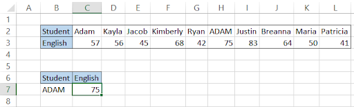
Suppose our dataset of students consists of two ‘ADAM’ - one in the upper case in cell H2 and the other in the normal case in cell C2.
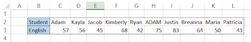
Assume that the teacher wants to know how many marks ‘ADAM’ scored on his English paper. For this, we will use a combination of MAX, EXACT, COLUMN, CHOOSE, and TRANSPOSE functions.
The EXACT function will compare two strings considering the case sensitivity of the strings and return TRUE if they match or FALSE if they don't match.
The TRANSPOSE function will change the orientation of the data, i.e., if it is in horizontal orientation, then it will change it to vertical data and vice versa.
The COLUMN function will return the column number based on the cell reference. In short, the combination of functions basically will change the table into vertically oriented data (upon which VLOOKUP is usually used) and return our result.
The formula we will be using to find the marks scored by ‘ADAM’ is =HLOOKUP(MAX(EXACT(B7, C2:L2) * COLUMN(C2:L2)), TRANSPOSE(CHOOSE({1,2}, TRANSPOSE(COLUMN(C2:L2)), TRANSPOSE(C3:L3))), 2, FALSE).
Since this is an array formula, you must press Ctrl + Shift + Enter to get the result and avoid the #N/A error.
This will give you the results as follows:
However, as you can see, the formula gets really complicated. The task is to make things easier for us while working so that it saves us time to look into other matters.
This is why, as much as we like going into depth while working on Excel formulas, we suggest that you use the combination of INDEX, MATCH, and EXACT functions.
The corresponding formula to achieve the same result is =INDEX(C3:L3, MATCH(TRUE, EXACT(B7, C2:L2), 0)):

We will break down the formula to help you understand what exactly is done here. First, the EXACT function looks into the range C2:I2 for the value ‘ADAM’. If it finds the value, the result will be TRUE or else FALSE.
Hence, the result for our EXACT function will be (FALSE, FALSE, FALSE, TRUE, FALSE, FALSE, FALSE) for all the values in range C2:I2. Now, the MATCH function will use TRUE as its lookup value and return the relative position for that value, which then will be used by the INDEX function having referenced range C8:I8 to give us the value 53, i.e., cell F8.
What formula to use for the case-sensitive HLOOKUP is entirely up to you and your tastes. If you go a long way, you might even stumble upon a better and simpler way than either of those!
Since this is an array formula, you must press Ctrl +Shift +Enter in the cell to display the result, or Excel will give an #N/A error (except in Excel 365).
You can read more about the INDEX MATCH formula here
Partial match using the wildcard characters
Wildcard characters help to return information from the database for text containing unknown characters and are helpful to locate multiple items in our database excluding the duplicates.
Before we go on to explain an example of partial match using wildcard characters, let us look at the different types of wildcards that you can use in the formula:
| Character | Explanation | Example |
|---|---|---|
| * | It matches the characters before * with text and returns all the strings. | he* will return hello, hell, hebrew but not chef, chew. It would have returned the latter words for che* |
| ? | It will match a single alphabet position of a text string. | bee? Will return beer, beep, beet, etc |
| [] | It will match characters within the square brackets | bee[rt] will return beer, and beet but not been |
| [ ] + ! | An exclamation mark followed by characters inside brackets excludes them from the text match | bee[!rt] will not return beer, beet but will return beep, been |
| [ ] + - | A range of alphabets(in ascending order) separated by a dash in brackets matches all the similar text in string | a[a-c]c will return aac, abc, acc |
| # | It will match numerical characters. | 2#2 will return 252, 212, 222 |
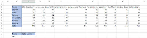
Let’s assume that the teacher knows the first three letters of her student’s name. She needs to know what are the total marks ‘Ari’ scored in her examination. The horizontal table for the dataset looks as below:
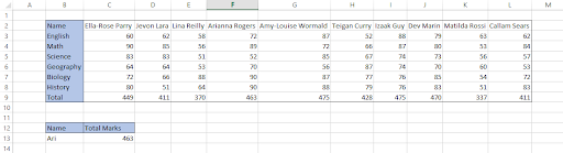
For this, the teacher can use the formula =HLOOKUP(B13&"*," C2:L9, 8, FALSE), which will match the value in cell F2 and return the value 463 in row 8 of our table_array based on the row_index_number assumption.
Concatenating the wildcard character without the quotation mark will result in an error while using the formula.
Return multiple values from HLOOKUP
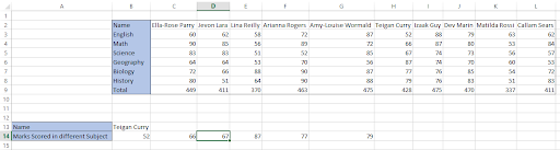
We have seen in previous examples how it is possible to pull Exact and approximate values. However, sometimes, you might be required to return all the values for a specific lookup_value. Let's say you need to return marks scored by Teigan in different subjects. The table looks as follows:

Here you need to modify your row_num_index argument by adding the row numbers in curly brackets, i.e., { }. The formula which will be used in returning the marks scored in different subjects is =HLOOKUP(B13, C2:L9, {2,3,4,5,6,7}, FALSE). Since this is an array formula, you must press Ctrl + Shift + Enter to return the result as below:
When you check the formula, you notice that your formula itself is enclosed in the curly brackets after pressing Ctrl + Shift + Enter for the array formula.
{=HLOOKUP(B13, C2:L9, {2, 3, 4, 5, 6, 7}, FALSE)}
Using this formula can be tricky, as you must first select the cells in which you are expecting the result.
For example, we selected the range B14:G14 and then entered/copied the formula in B14 and finally ran the array formula to give the result. You might get an error the first time, but you will definitely get a hang of this once you understand how the formula works!
Conclusion
Excel's HLOOKUP function is a useful tool for finding and obtaining data from tables or arrays that are arranged horizontally. Data analysis and manipulation operations are streamlined by its capacity to locate values in the top row of a dataset and retrieve corresponding values from specified rows below.
Through a thorough comprehension of the data structure and exact specification of parameters like the table array and row index number, users may fully utilise HLOOKUP's capabilities to effectively extract precise information.
Furthermore, selecting between approximate and exact match types increases flexibility to accommodate various data circumstances.
Adopting HLOOKUP enables users to effortlessly traverse through sizable datasets, promoting well-informed decision-making and augmenting efficiency across diverse domains such as finance, project management, and data analysis.

Everything You Need To Master Excel Modeling
To Help You Thrive in the Most Prestigious Jobs on Wall Street.
Free Resources
To continue learning and advancing your career, check out these additional helpful WSO resources:


or Want to Sign up with your social account?