MATCH Function
An Excel Lookup and Reference function looks for a specified value within a range of cells and returns the relative position of the value in the referenced field of cells.


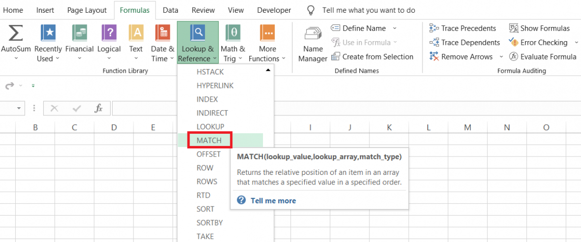
What is the MATCH Function?
The MATCH function is an Excel Lookup and Reference function that looks for a specified value within a range of cells and returns the relative position of the value in the referenced field of cells.
The easiest way to understand how the function works is through dating websites such as Tinder.
When you create an account, the platform might ask you a few questions about what characteristics you want in the person, such as age, degree of commitment to a relationship, etc.
Based on the inputs, the platform works out a list of possible matches and may display a message such as ‘10 matches found’.
The MATCH function works similarly. It replaces the characteristics with a data type, such as text strings, numbers, dates, or even times, and checks the referenced data for an exact match.
This article will see the MATCH function, its syntax, workings, and some examples.
- The MATCH function in Excel searches for a specified item in a range of cells and returns its relative position.
- An alternative to the MATCH function is the XMATCH, which also returns the position of value from a given range.
- MATCH is helpful for looking up list values, comparing lists, and finding specific data in large datasets.
- It's commonly used with other functions like INDEX to retrieve values from a list or table based on their positions.
Understanding the MATCH function
The MATCH function is categorized as a Lookup and Reference function that returns the relative position of a value within an array.
The function looks up both ‘exact’ and ‘approximate’ matches and returns their relative position from a range of values.
For example, suppose that you need to find the value ‘John.’ The values in the array are Jim, Jason, Jacob, John, and Jonathan. When the MATCH function is used, it returns the result as 4, meaning it found a match at the fourth value in the array.
On a closer look, we find that the fourth value in the array is ‘John’ and that both the input and output values match each other.
The function is even capable of finding a match using a wildcard character. For example, if you have the array of John, Marsh, and Nick and the lookup value is ‘Jo,’ it will still find an equivalent value from the display, which in this case is ‘John.’
MATCH function Formula
The syntax for the function is:
=MATCH(lookup_value, lookup_array, [match_type])
- lookup_value - (required) the value we are looking for in the lookup_array. For example, when looking at the subway timings, we use the train’s identification number to determine when the train will arrive at the platform accurately.
- lookup_array - (required) the range of cells evaluated for lookup_value
- match_type - (optional) determines the match type. It can be one of the three values from -1, 0, and 1. If the argument is skipped, Excel accepts 1 as the default value.
| match_type | Behavior |
|---|---|
| 1 | The function finds the largest value less than or equal to the lookup_value when the lookup_array is in ascending order. |
| 0 | The function is able to identify the first value that is an exact match from the lookup_array irrespective of the orientation of data. |
| -1 | The function finds the largest value less than or equal to the lookup_value when the lookup_array is in descending order. |
How to Use the MATCH Function in Excel
It is easy to interpret what we need to do for lookup_value and lookup_array. But what about match_type?
In the earlier section, we read that the match_type argument can only accept three values, but each value can be used only based on predefined criteria.
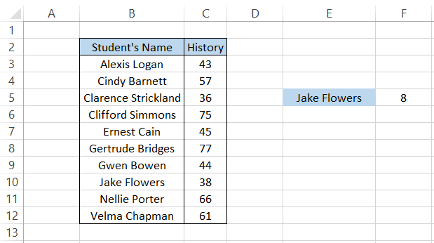
Suppose that you have the data as illustrated below:
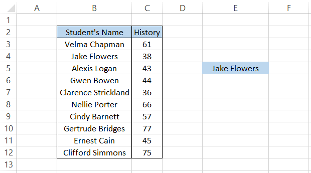
Lookup_value
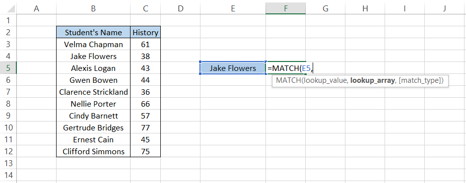
We want to find the position of ‘Jake Flowers’ in the given dataset. The first argument in the function is the lookup_value which is present in cell E5. The formula becomes
=MATCH(E5, lookup_array, [match_type])
as illustrated below:
Lookup_array
The lookup_array is the range of values wherein we must check if the lookup_value exists. Our lookup_range is in column B (i.e B3:B12) such that the formula becomes
=MATCH(E5,B3:B12, [match_type])
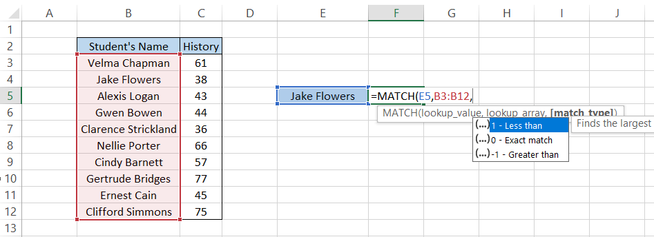
Match_type
This is where things get a bit tricky. Here, the value of utmost importance for the match_type argument is 0. If you input the value as 0, then the MATCH function finds an exact match from the lookup_array.
The formula becomes
=MATCH(E5,B3:B12,0),
giving a result of 2. This is the position where you would find ‘Jake Flowers’ in the range B3:B12.

But what about the other two values? As we said earlier in the function’s syntax, the value 1 is used when the lookup_array is ascending, while -1 is used when the lookup_array is in descending order.
If the values in the array are not in either ascending or descending order, then the function might return confusing results using the MATCH function.
Example Of MATCH Function
For example, let’s say we use the formula
=MATCH(E5,B3:B12,1)
in cell F5, which gives the result as 10. But it’s not possible since the current position for ‘Jake Flowers in the given dataset is 2.
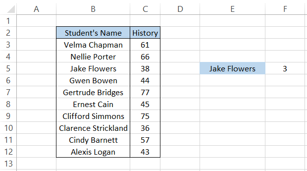
However, if you sort the range B3:B12 in ascending order, we get:
Since the data is now sorted from A to Z, we find that ‘Jake Flowers’ is in the 8th position, which makes more sense now. Similarly, if the data were organized from Z to A direction, the position for ‘Jake Flowers’ would be 3.
The formula would also change to
=MATCH(E5,B3:B12,-1)
where the table would look as illustrated below:
The same logic can also be applied to numbers, and the match_type argument can be assigned accordingly to return the position for a particular lookup_value.
INDEX MATCH function
There’s even a chance that you might never have heard of this fantastic combination of functions that supersedes both VLOOKUP and HLOOKUP functions.
However, the only drawback to the formula is that most people find it rather tricky to use and interpret when compared to the VLOOKUP function.
The formula consists of two functions: INDEX and MATCH. The INDEX function is categorized as a Lookup and Reference function that returns a value in a given array based on the row and column numbers.
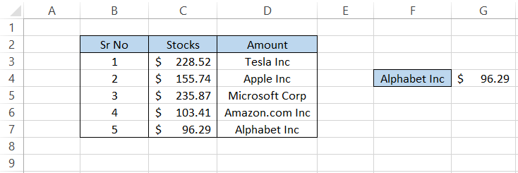
Let’s say that you have the stock price data as illustrated below:
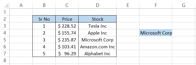
If we were to extract the price for Tesla Inc, the array would be D3:D7 while the row and column numbers would be 1.
Both the row and column numbers are 1 since there is just one column in the referenced range, while the ‘Tesla Inc’ is in the first row of the data itself.
Formula
The syntax for the INDEX function is
=INDEX(array, row_num, [column_num])
where,
- array - (required) range of cells from which the required value will be returned. The subsequent row_num and column_num arguments are optional if the array consists of a single row and column.
- row_num - (required) the row number from which the function extracts the value. The column_num argument is required if the row_num fight is skipped.
- column_num - (optional) the column from which the function extracts the value. This argument can be skipped if the required value is only based on the row_num opinion,
So how do INDEX and MATCH come together? We already know that the latter function returns the position of a lookup_value within a lookup_array in number form.
Based on that, the numbers are then used as the row_num and column_num arguments, which finally retrieve a value from the referenced array using the INDEX function.
If we wanted to extract the price of Alphabet Inc., the formula would be
=INDEX(C3:C7,MATCH(F4,D3:D7,0))
giving the result as $96.29.
We have dedicated an example to the INDEX MATCH function that will provide you with various use cases for the functions and explain why the combination is far superior to the traditional VLOOKUP and HLOOKUP.
Note
Even after a couple of tries, if you still find the combination a bit difficult to use, Excel also recently introduced the XLOOKUP function, which offers greater versatility but is simpler to use.
MATCH function Example
Now that we know how to use the function, let’s see another simple example before we proceed to the tricky combo of INDEX MATCH.
Suppose that you are a day trader and make a series of investments as illustrated below:
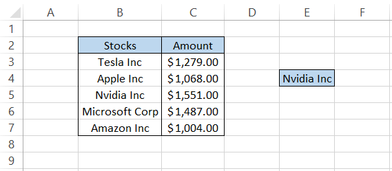
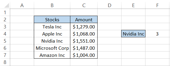
To get the position of Nvidia Inc. stock in the given dataset, we will use the formula
=MATCH(E4,B3:B7,0)
in cell F4, which gives the result as 3.
However, we can hardly do anything with just the position returned by the formula.
What if we told you that you could return the corresponding amount you spent on the stock based on the position returned?
This is possible using the combination INDEX MATCH, which returns the value corresponding to the ‘matched value’ from the given dataset.
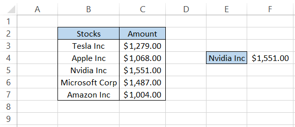
For example, if we wanted to return the amount from column C for Nvidia Inc., placed in the third position, a glance of eyes would say that the amount is equal to $1,551.00
But what if you had thousands of rows of data?
In this case, we will use the formula
=INDEX(C3:C7,MATCH(E4,B3:B7,0))
in cell F4, which gives the result of $1,551.00
The INDEX MATCH is considered an upgrade over the VLOOKUP and HLOOKUP functions since it offers a lot more versatility and covers the shortcomings of the latter parts.
MATCH vs. XMATCH
If you have been using a recent version of Excel, you might have noticed another function similar to the one on which the article is based- the XMATCH function.
XMATCH is a new-gen function that returns the relative position of the specific item in a referenced range of cells.
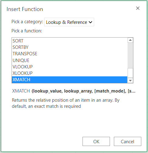
This new function is an upgrade to its predecessor, the MATCH function.
The syntax for the function is:
=XMATCH(lookup_value, lookup_array, [match_mode], [search_mode])
Where,
- lookup_value - (required) the value that the user is searching for. For example, when buying stocks from a broker app, we usually type in the ticker symbol or the stock name to identify it from the given list.
- lookup_array - (required) the data which will be evaluated to find the lookup_value
- match_mode - (optional) allows the user to find an exact or an approximate match.
Depending on the requirement, match_mode can take different values:
| 0 | Finds an exact match only when the lookup_value exactly matches the value in lookup_array. |
| -1 | Finds the next smallest value from the lookup_array in case Excel isn’t able to return an exact match. |
| 1 | Finds the next largest value from the lookup_array in case Excel isn’t able to return an exact match. |
| 2 | Allows the use of wildcard characters, like asterisks (*) and question marks (?) for partial matching |
- search_mode - (optional) determines the directional orientation in which the function must find the value in the lookup_array.
The different acceptable values that can be used are:
| 1 | By default, the function searches for the lookup_value in the lookup_array from the top to bottom direction. |
| -1 | Excel iterates through the data from bottom to top in the lookup_array. |
| 2 | The lookup_array is arranged in ascending order for a binary search. |
| -2 | The lookup_array is arranged in descending order for a binary search. |
The two major differences between the functions are the inclusion of match_mode and the search_mode arguments in the function. Respectively, these arguments return the exact or approximate matches and let the user look at data from top to bottom or vice versa.
Example
Let’s see an example to understand how the optional arguments work using the XMATCH function. Suppose that you have the data as illustrated below:
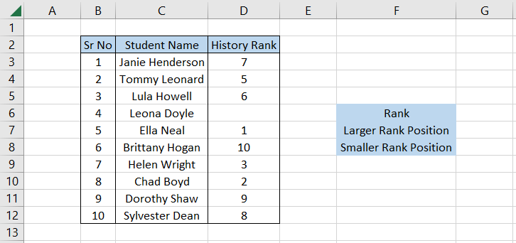
Let’s assume that we need to find the position of one rank higher and lower than 4 in the lookup_array D3:D12.
As you might have noticed, we are missing rank 4 in the given dataset. By using the formula
=XMATCH(G4,D3:D12,1)
we can find the position of one rank higher, whereas the formula
=XMATCH(G4,D3:D12,-1)
finds the part of one rank lower than 4.
We get results 2 and 7 as the positions for more extensive and minor ranks, respectively.
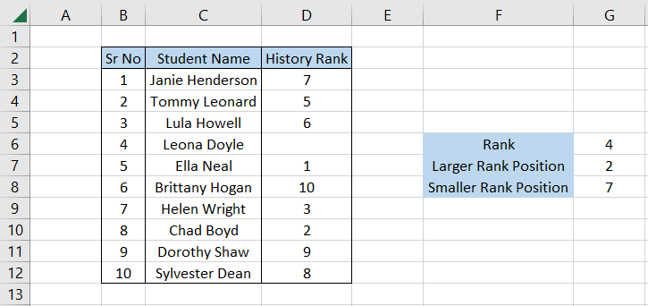
This means that a rank larger than 4 is present in the second cell in the array D3:D12, which ranks 5. Similarly, a level lower than 4 is present in the array's seventh position, rank 3.
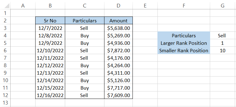
Similarly, the search_mode allows one to look for a value from either top to bottom or vice versa. Suppose that the data is as illustrated below:
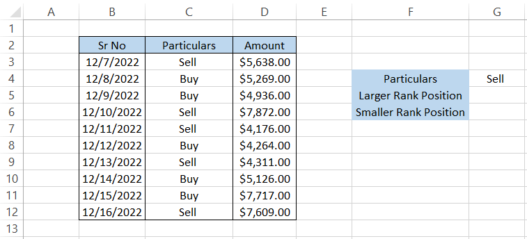
If we want to find the first ‘Sell’ transactions from top to bottom, we will use the formula
=XMATCH(G4,C3:C12,0,1),
which gives the position as 1.
Similarly, the first ‘Sell’ transaction from the bottom to the top will be returned using the formula
=XMATCH(G4,C3:C12,0,-1),
which gives the position as 10.
You can even combine the XMATCH function with the INDEX to return customized results, which is impossible with the INDEX MATCH combination.

Free Resources
To continue learning and advancing your career, check out these additional helpful WSO resources:


or Want to Sign up with your social account?