TRANSPOSE Function
An Excel Lookup/Reference Function that allows you to switch the orientation of a data array or a given range, i.e., from horizontal to vertical and vice versa.


What Is The TRANSPOSE Function?
The TRANSPOSE function is an Excel Lookup/Reference Function that allows you to switch the orientation of a data array or a given range, i.e., from horizontal to vertical and vice versa.
![]()
This change of data array from vertical to horizontal and vice versa can help users reorganize and manipulate data efficiently. The function is particularly helpful when there is a need to present the data in different layouts and formats.
This streamlining of data aids in data analysis, data presentation, and enhancing the overall data efficiency in Excel
A helpful analogy to understand how the function works is by comparing it to playing jigsaw puzzles.
Just like when we come across a piece that we feel is the correct one, we try to orient and rotate it in all four possible ways to fit it into a bigger picture. Based on its existing orientation, it can ‘flip’ an array or data in a horizontal or vertical direction.
The most important thing to remember is that it is an array formula. An array formula can perform one or more calculations on multiple items in the referenced array.
To get a better grasp of what the function does, let's observe it in action. In this article, we will see the TRANSPOSE function, its syntax, and a couple of examples to understand it better.
- The TRANSPOSE function is categorized as a lookup and reference function that flips the orientation of the given dataset.
- The syntax for the TRANSPOSE function is simple. It typically requires only one argument: the range of cells you want to transpose. It returns a new range of cells with the data flipped.
- The TRANSPOSE function is helpful in scenarios where you need to reorganize or reshape data, such as switching between different views of a dataset, creating summary reports, or preparing data for charts and graphs.
- The TRANSPOSE function has limitations regarding the range size it can handle. It can only transpose data within a single worksheet, and the number of rows and columns in the transposed range cannot exceed the maximum limits allowed by Excel.
How TRANSPOSE Function Works?
It is classified as a Lookup and Reference function that allows you to switch the orientation of an array. By referencing the range of cells in the function, it effectively ‘flips’ the horizontal array into a vertical array and vice versa.
![]()
When the data is in vertical orientation, and you apply the TRANSPOSE function, the first column becomes the first row in the array, the second column becomes the second row, and so on.
Similarly, if the data is in horizontal orientation, the first row becomes the first column, the second row becomes the second column, and so on, until the end of the rows.
The syntax for the TRANSPOSE function is:
=TRANSPOSE(array)
where,
- array - (required) range of cells whose orientation will be changed from horizontal to vertical and vice versa.
NOTE
Transposed arrays are dynamic in nature. For example, if you change any of the values in the original data source, it will also automatically reflect in the transposed data.

How to use the TRANSPOSE Function?
Now, here comes the tricky part. You all are probably thinking, “How difficult would using the TRANSPOSE function be, right?”
![]()
Well, it's not difficult if you know the correct instructions. However, the initial step is where many mistakes can be easily made.
Let’s break down the process of using it in two steps:
1. Selecting the target range
Assume you have the data as illustrated below:
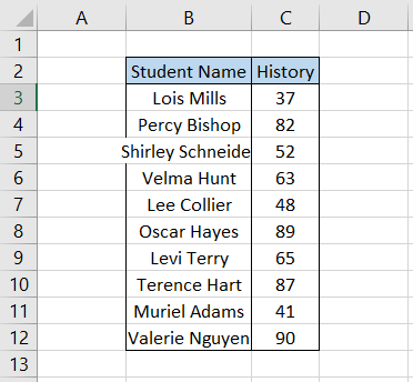
As you can see, the data is in vertical orientation. However, after preparing the data, I believe it would be easier to maintain the test scores in the horizontal orientation.
Should I make the table again?
Absolutely not. All you need to do is first select the range in which you expect the transposed data. It doesn’t matter if you select additional cells; those cells will return a #N/A error if the value is missing.
![]()
Once the target range is selected, by using it the formula becomes =TRANSPOSE(B3:C13) in the first cell of the target range as illustrated below:
![]()
2. Pressing the Shift + Ctrl + Enter key
Now that you are done with the difficult part, let’s come to the easiest step left to return the data in horizontal orientation.
Once you have typed in the formula, you must press Ctrl + Shift + Enter to get the result since this is an array formula. We will get the data as follows:
![]()
It will not work if you do not press those keys in Excel 2019 and lower versions. However, if you use the Excel 365 version, you don’t need to select the target range or press the Ctrl + Shift + Enter key.
Excel 365 supports the use of dynamic array formulas, and thus you can directly type in the formula in any cell without selecting the target range to give the result.
Since the result returned using the TRANSPOSE function is dynamic, any changes you make in the original table will be automatically reflected in the ‘transposed’ data.
For example, if we change Percy Bishop's test score to 90, the value in the ‘transposed’ data also automatically changes to 90.
Thus, you need to be extremely careful if you think of changing any numbers in the original table since it will directly reflect in the transformed table.
Example of the TRANSPOSE Function
Let’s see a couple of examples to understand further how the TRANSPOSE function works and how you can maximize its potential while working on datasets.
A) Simply transposing the data
If the objective is to transpose the data simply, we select the target range and then use the TRANSPOSE function.
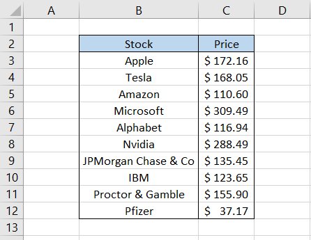
We see that our data has two columns and eleven rows. Thus, the target range would also have two columns and eleven rows. We will select the range and type in the formula =TRANSPOSE(B2:C12) in the first cell as illustrated below:
![]()
The final step is to press the Ctrl + Shift + Enter key, which will return the result as:
![]()
Since this is an array formula, you cannot delete the value from a single cell. This is only possible when you delete the data from the entire table.
B) Transposing empty cells
One of the issues with transposing the data consisting of empty cells is that the TRANSPOSE function will automatically change those empty cells into numerical value zero.
For example, suppose you have the data as illustrated below. We see that the price for Tesla, Microsoft, and JPMorgan Chase & Co is missing from the table.
![]()
If we transpose the data directly, all the empty cells will return the value as zero. The problem is we want to update those numbers later and thus need the cells to remain empty.
To retain the original cell value, we will use the formula =TRANSPOSE(IF(B2:L3="","",B2:L3)) after selecting the target range as below:
![]()
Now, all you need to do is press the Ctrl + Shift + Enter key, and you will get the result:
![]()
As you can see, all the empty cells are retained in our transposed dataset. So the formula is really simple - we just add a conditional formula to check if the array of cells has any empty cells.
If such cells are found, they are ‘required’ to return as empty cells. If there are no empty cells, the function will return whatever values the cell possesses.
The use of the IF function allows you to return empty cells as well as any other customized text string easily.
C) Retrieving data based on multiple parameters
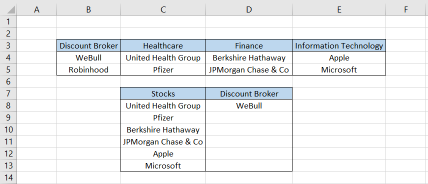
Suppose you invest in two different platforms - WeBull and Robinhood. To build a diversified portfolio, you invest in Healthcare, Finance, and Information Technology.
The trading data and the stocks that fall in those particular buckets are illustrated below:
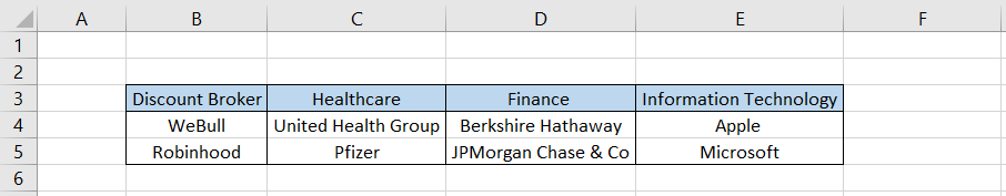
Thus, while interpreting the data, you can say that Pfizer, JP Morgan Chase & Co, and Microsoft were purchased on the Robinhood platform, while other stocks were purchased on the WeBull platform.
However, what if we had thousands of rows and columns of data?
How difficult would it be to retrieve the discount broker or even the corresponding sector for each invested stock?
In this case, we can use a complicated formula to return the discount broker for the corresponding stock in a single transposed table.
First, copy all the unique stocks in another range, C9:C14, as illustrated below:
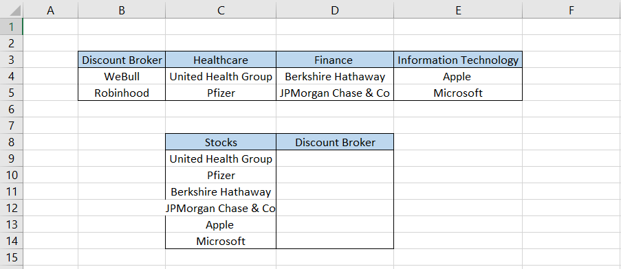
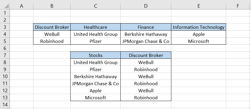
To return the discount brokers in range D9:D14, we will use the formula
=INDEX($B$4:$B$5,MATCH(-1,MMULT(-($C$4:$E$5=C8),TRANSPOSE(COLUMN($C$4:$E$5)^0)),0)) in cell D9 and press the Ctrl + Shift + Enter key to get the result:
To get the rest of the discount brokers, we will drag the formula down till cell D13 as illustrated below:
As you might have noticed, we did not select the target range but dragged the formula down until the last cell. This is because the formula comprises several different functions, which we will try to break down to understand better.
- Firstly, the formula COLUMN(C4:E5) finds the number of columns in the range C4:E5 equal to 3. When this number is raised to the power of zero, the result ultimately is 1, which is what we are seeking for creating a single-column dataset.
- When you transpose this number using the formula, =TRANSPOSE(COLUMN($C$4:$E$5)^0), the result remains 1 with an array of {1,1,1}.
- Another part of the formula is the $C$4:$E$5=C8, which creates an array of ‘1’ and ‘0’ based on the presence of the stock in the range. For example, the array for UnitedHealth Group becomes {1,0,0,0,0,0}.
- When you use the MMULT function using the formula MMULT(-($C$4:$E$5=C8),TRANSPOSE(COLUMN($C$4:$E$5)^0)), it multiples the array returned from both the output to give a final array of {1,0}.
- This returns the position of a discount broker, i.e., either B4 or B5 in the referenced cell.
- The formula may look a bit complicated but is nevertheless handy when returning the dataset to its one-dimensional counterpart.
That should probably suffice in understanding the TRANSPOSE function better!

Free Resources
To continue learning and advancing your career, check out these additional helpful WSO resources:


or Want to Sign up with your social account?