LEFT Function

What is the LEFT Function?

The LEFT function in Excel extracts the 'n' number of characters from the left side portion of the text string. 

Excel has offered several text manipulation functions to all the users in the Excel community. For example, the MID and RIGHT function have been immensely used to extract text from a text string's middle or right side. So what are the different scenarios you can think of when we say by extracting a substring?

This could include getting the zip codes from the end of the address(using RIGHT), states or cities (using the MID function), and finally, the street address(using the LEFT process).

Even though the function works amazingly on its own, it can combine with other functions, such as SEARCH or FIND to take text manipulation up to another level.

In this article, we will understand the function's syntax and explore different examples to help us understand the part better. 

Understanding the LEFT function

The LEFT is categorized as a text function that will extract a specified number of characters from the left side of the string.

Now you would ask which left side - is it ours or the system we are working on? 

The answer is you. In simple terms, you can also say that the function will extract a substring from the starting position of a text string.

For example, if you have the text string as "Technical Analysis," you can obtain 'Technical' as a substring while ignoring all the unnecessary characters present after our substring.

However, to extract the substring, we must first-hand know the end position of the substring or how many characters to remove. We can do this by counting the number of characters, which gives us the count of characters in the substring 'Technical' as 9.

If you had used the count of characters as 10, the function would have extracted the space between the two words since Excel also counts space as a character.

The syntax for the LEFT function:

=LEFT(text,[num_chars])

where,

• text = (required) The text string from which you intend to extract the characters
• num_chars = (optional) The number of characters to extract from the text. If you skip the argument, the function takes in the default value of 1, meaning it will only obtain one character.

How to use the LEFT function?

There are two different methods at your disposal to use the function. Either way will ultimately give you the same result, so it is really up to you what method you choose.

a) Method #1: From the function's library

Functions are what you can call pre-established formulas, where you need to input the arguments in the dialog box to get the result in the desired cell directly. To use the LEFT function, please follow the steps given below:

1. Before using the function, an important step is to select the cell in which you intend to get the result. For example, if it's cell B3, then select the same cell.
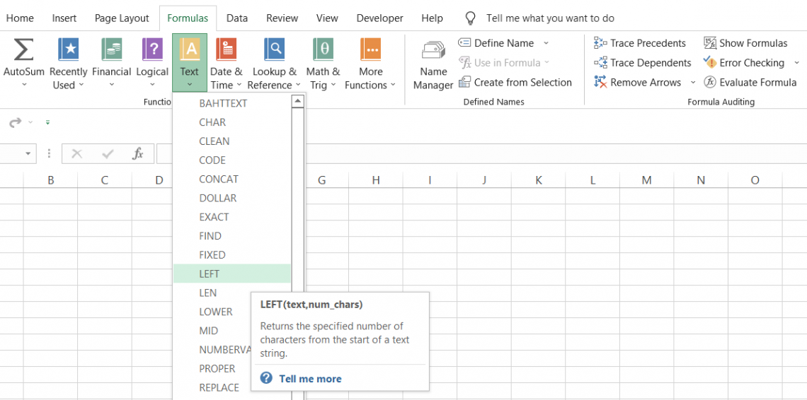
2. Click on the Formulas Tab > Text > and then click on the LEFT function.
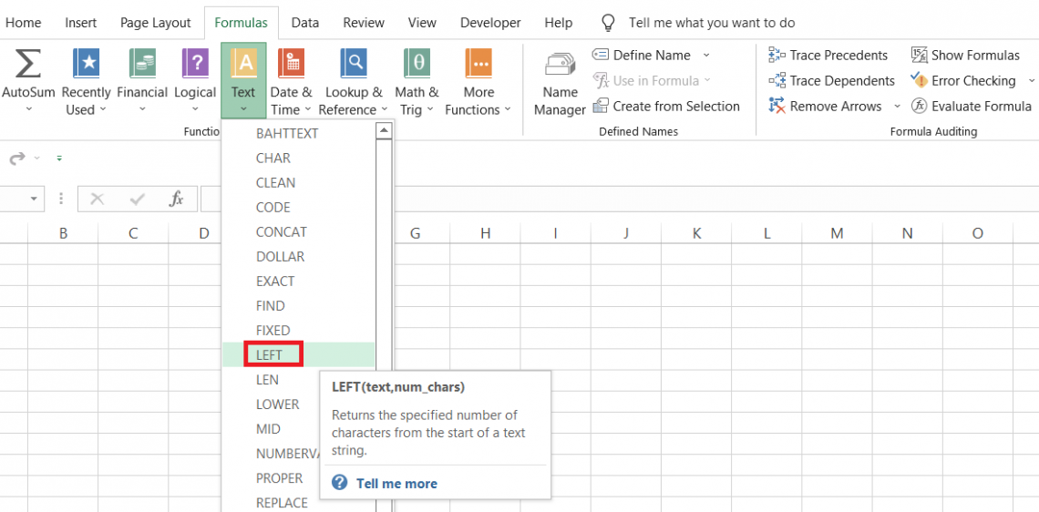
3. This will open up the function's dialog box, as illustrated below:
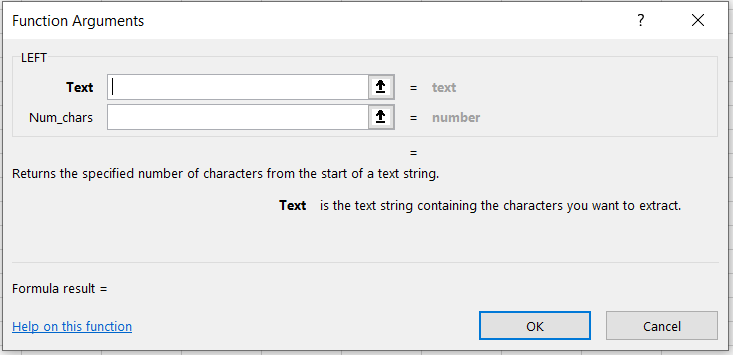
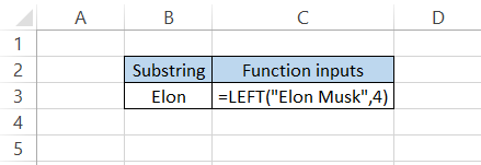
4. Next, we input the arguments in the dialog box. For example, if the text is 'Elon Musk' and we intend to extract the substring 'Elon' consisting of 4 characters, then the num_chars will be 4.
   Don't forget to use quotation marks since our required argument is a text string. Once you input both arguments, you should get a preview of what your expected result would be.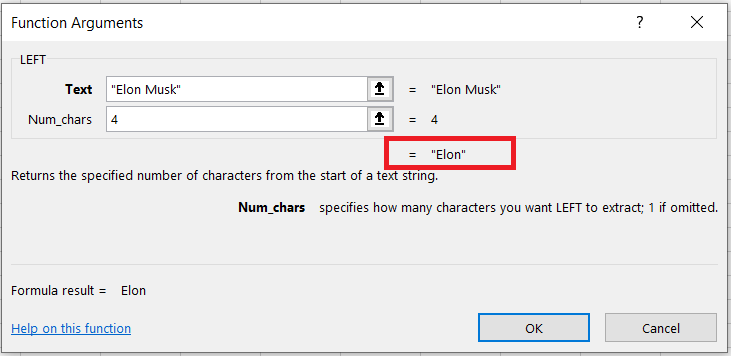
5. When you click on Ok, you will get the same result in the selected cell, as illustrated below:
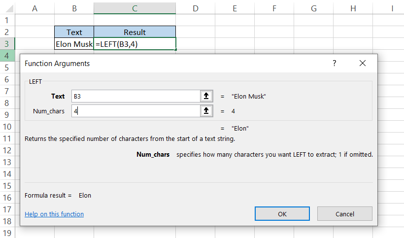
6. You can also directly input the cell references to 'text strings' in the function, giving you the same result.

b) Method #2: As a worksheet function

To use the function as a worksheet formula, you begin with an equal sign and input the function name followed by the arguments inside the parenthesis.

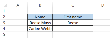
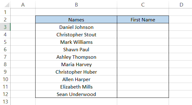
Let's say you want to extract the first name from the full name of one of your customers.

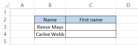
To extract the first name 'Reese' in cell C3, we will use the formula

=LEFT(B3,5),

which should give you the result as illustrated below:

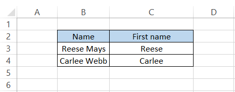
We knew that the first name 'Reese' had five characters and used the num_chars as five. But what about the next name on our list?

Can we drag the formula down in cell C4 and expect a similar result?

We have saved this for one of the sections below, so please ensure that you remind us!

Returning to our first name for cell C4, we need to manually input the num_chars as 6 so that the formula is =LEFT(B4,6) to give you the result as 'Carlee.'

Examples of lEFT Function

Let's begin with a simple example and make our way to the following levels to understand how the function works independently and in combination with other parts.

a) Example #1 

Suppose that you need to extract the street name from the complete address. The address that you need to manipulate is, as illustrated below:

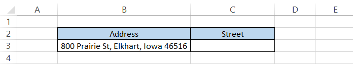
Upon closer inspection, we can conclude that the address is represented in Street/City/State/Zipcode format. That means we only need to extract the substring ‘800 Prairie St' as our result in cell C3.

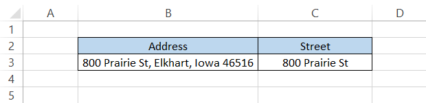
We will count the characters(including the spaces), which equals 14. Thus, our formula to return the street will be =LEFT(B3,14), which will give you the result:

b) Example #2

Let's agree that counting the characters for each text string is inefficient. Assume there are a thousand rows of data, and you need to separate the street names or the first name from each cell where each substring is of varying length.

That's where the SEARCH or the FIND function comes in. 

Both functions have the same syntax:

=SEARCH(find_text, within_text,[start_num])

or,

=FIND(find_text, within_text,[start_num])

where,

• find_text = (required) the substring that we intend to search for in the text string 
• within_text = (required) the text string which will be searched for the substring
• start_num = (optional) the starting position within the text string.

For example, suppose you have the text string as 'Jeff Bezos' and need to find the position of the first 'e,' we will input a start_num as 1(starting position), which should give you the position for 'e' as 2.

Either function helps extract a substring based on a 'delimiter' presence. A delimiter is a character that separates text strings by forming a boundary between them.

Some of the common delimiters between the text strings are space, commas( , ), semicolons( ; ), a pipe/ vertical line ( | ), or the back and front slashes (/ \).

Returning to our example based on names, assume that you have different terms of varying lengths from which you need to extract the first names.

Here, we will use the combination of LEFT and SEARCH functions to find the space delimiter and extract the first names.

The formula will be

=LEFT(B3, SEARCH("", B3)-1),

which will give you the following result:

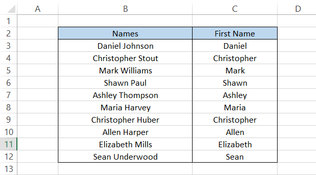
Firstly, why did we subtract 1 from the formula? The reason is that since we searched for the 'space' character, the formula also includes it in our result. 

The result you are getting is 'Daniel' + 'space character,' and we subtract it from the corresponding number to remove it. Another alternative is the TRIM function, which will remove all the unnecessary spaces from your substring once you extract it successfully.

As you can see through our entire result, the substrings are of varying lengths, yet we were able to obtain the first names accurately. This could be achieved with the help of the delimiter that was present in the dataset.

c) Example #3

There is another function that you can use in combination with the LEFT, which is the LEN function.

Suppose you receive specific data with recurring fixed-length characters at the end of the text string. The example for the dataset is illustrated below:

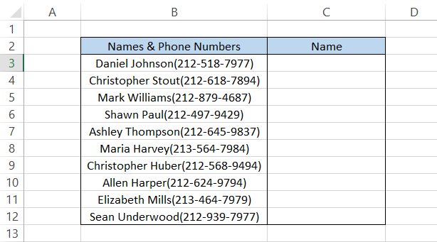
We can see that the name is always followed by the phone numbers between the opening and closing parenthesis. The total number of characters apart from the title equals 14 in each row.

To separate the name from the phone numbers, we can use the formula

=LEFT(B3, LEN(B3)-14)

in cell C3 and drag it down to cell C12. This will give us the result:

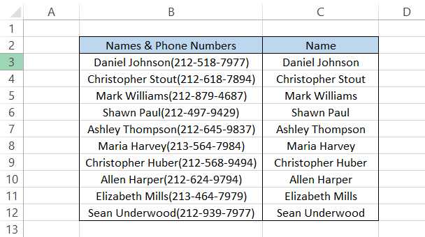
It doesn't matter if the text string separated by delimiter is of varying length at the beginning. However, the characters you want to trim in the dataset must be the same length.

Apart from this downside, we don't see any reason you shouldn't use the combination of LEFT and LEN functions to take your data analysis skill to the next level.

d) Example #4

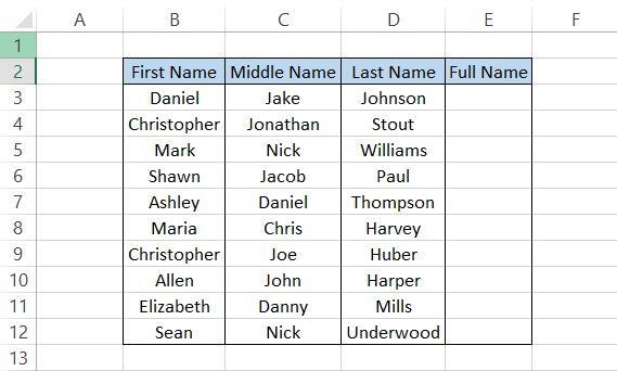
Suppose you receive a file with First Name, Middle Name, and Last Name in separate columns. However, your system only accepts them as one value separated by delimiter period (.), and on top of that, the Middle Name should have just the length of one character.

How would you get the final value say, as Monkey.D.Luffy?

The data can be seen as

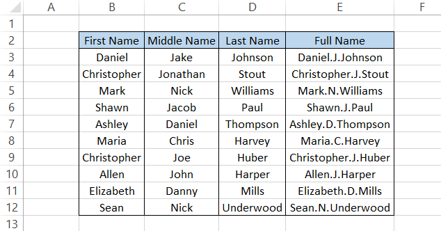
To get the result in our desired format, we will use the formula

=B3&"." &LEFT(C3,1)&"."&D3,

which will give you the result as 

If any components in the full name are in lowercase, we can use the UPPER function that will return the first letter of the text string as capitalized.

You could also use the CONCATENATE function instead of '&'. However, we prefer to use it since it is easy to include in the formula!

Practical Example - Extracting text up to Nth word

By now, you understand that the function will extract all the substrings with a character's length less than the entire substring and only from the left side of the beginning of the string.

In our article on the MID function, we saw how you could extract a word present in the 'nth' position based on the number you input for its role in the text string.

On the other hand, in this article, we will see how you can use the combination of LEFT, SEARCH, and SUBSTITUTE functions to extract a substring up to an 'nth' word in your sentence.

Suppose that you have the text string below:

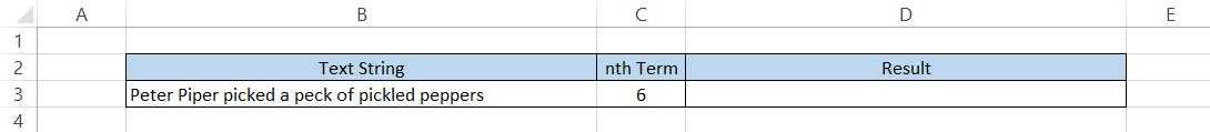
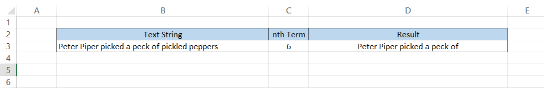
To extract the substring up to the 6th word, we will use the formula 

=LEFT(B3, SEARCH("@", SUBSTITUTE(B3," ", "@", C3))-1),

 which will give us the result as 

If we change the 'nth' term to 2, then the formula returns the result that has only two words in the substring, as illustrated below:

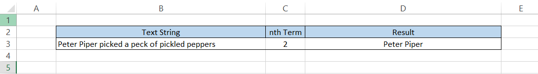
To understand the formula better, we will break it down into three parts:

a. SUBSTITUTE function - Being the innermost function nested in the formula, the SUBSTITUTE function finds the 'space' character after the 'nth' word inside the text string and replaces it with the '@' character

So if we have the nth term as 3, then the third instance of 'space' will have its character replaced by a '@'. All the other space characters in the sentence would be unaffected.

b. SEARCH function - Once the SUBSTITUTE function has worked its magic, the formula then uses the SEARCH function to find our '@' character. By doing this, we ask the procedure to extract all characters to the '@' nature.

c. LEFT function - Finally, the superstar of our article takes in the text string as one of the arguments, while the num_chars argument is provided in the form of length until the '@' character

Thus, when you run the formula, we get a substring that is only up to the nth term specified in cell C3.

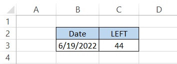
Date/Time and LEFT function

We know that dates are stored as serial numbers in Excel. So, for example, if the date is 19th June 2022, the serial number corresponding to the date would be 44731. 

Let's say you want to extract the date using the LEFT function. Naturally, you would expect the process to return the characters as 19 if you use the formula as 

=LEFT(C3,2).

However, the formula returns the result as 44, the first two serial number characters corresponding to the date in question.

Even when you are extracting time, the function works similarly since even time is stored as numbers or, more precisely, decimal numbers.

If you have the time as 11:31 PM, then the equivalent decimal number for the time would be 0.97986111111111. In this case, if you use the formula 

=LEFT(B4,3),

the result would be 0.9.

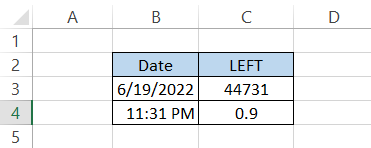
Don't forget about the period symbol(.), Excel will also count it as a valid character, which gives us the three characters as 0.9. 

Researched and Authored by Akash Bagul | Linkedin

Reviewed and edited by Parul Gupta | LinkedIn

Free Resources

To continue learning and advancing your career, check out these additional helpful WSO resources:

• FV Function
• PEARSON Function
• SEARCH Function
• SUBTOTAL Function
• YIELD Function