XLOOKUP Function
Returns a value from a different row or column by checking if the value matches a particular row or column


What is XLOOKUP?
The XLOOKUP is a Lookup/Reference function that returns a value from a different row or column by checking if the value matches a particular row or column.

If you have been using the INDEX MATCH function a lot, you will love it since it is much easier to use and gives you the same results.

For example, if you need to find what salary Josh earns each month, you can use the XLOOKUP function to return the result in a different cell. Unfortunately, as of now, the function is only available to Excel 365 users.
If you use any other Excel versions, you probably won't be able to use this function. But wait! That shouldn't stop you from learning this great function. We have a hack for you - head to Office 365 and open Excel online.
If you already own Excel 365 and are still unable to access it, click on the File tab and then on Account. There you will find the Office Insider program, which, if selected, will give you access to use the function in Excel.
The XLOOKUP function was the newest addition to Excel's capabilities when it was introduced in 2019 as a successor to the VLOOKUP and HLOOKUP functions.
The function can be used on vertically- and horizontally-oriented tables, search to the left, return multiple criteria, or even return the whole range of cells altogether.
This next-generation lookup function does not require the lookup value in the first row or column and can return a default value in case Excel cannot find the matter instead of an #N/A error.
- XLOOKUP is a powerful Excel function introduced in 2019, replacing VLOOKUP and HLOOKUP. It can work with vertical and horizontal tables, return multiple criteria, and handle whole ranges of cells. It doesn't require the lookup value in the first row or column and can provide a default value when a match is not found.
- The XLOOKUP function has a specific syntax: `=XLOOKUP(lookup_value, lookup_array, return_array, [if_not_found], [match_mode], [search_mode])`. You can use these parameters to customize your lookup.
- Using XLOOKUP is relatively straightforward. You start by defining the lookup value, lookup array, and return array. You can also handle cases when the value is not found using the `if_not_found` parameter. Additionally, you can fine-tune matching and searching behavior with the `match_mode` and `search_mode` parameters.
- The article provides practical examples of XLOOKUP usage, such as wildcard matching, left lookups (finding data to the left of the lookup value), finding the last occurrence, returning multiple rows or columns, two-way lookups, and conditional lookups. These examples demonstrate the versatility of the XLOOKUP function.
- XLOOKUP offers several advantages over its predecessors, including simplicity, default exact matching, automatic handling of missing values, flexible search directions, and faster processing, particularly for large datasets. It reduces the likelihood of errors and simplifies complex lookup operations.
XLOOKUP Function Syntax
The syntax for the function is:
= XLOOKUP(lookup_value, lookup_array, return_array, [if_not_found], [match_mode] , [search_mode])
Where,
lookup_value = the lookup value that you want to search
lookup_array = the array where you want to look at the value for
return_array = the array from which you want to return the value
if_not_found = This is an optional parameter that is returned if Excel cannot find the lookup_value. If ignored, Excel will return the #N/A error for missing values.
match_mode = Another optional parameter that specifies the match type for the function. The different values that can be used for match_mode are:
| 0 | This is the default option that finds an exact match in Excel. The lookup_value must exactly match the value in lookup_array to return the value. |
| -1 | Returns the next smallest value if Excel does not find an exact match. |
| 1 | Returns the next largest value if Excel does not find an exact match. |
| 2 | This option lets you use wildcards such as an asterisk( * ), question mark (?), etc. for partial matching |
search_mode = This parameter specifies how the function should look for the value in lookup_array and is an optional parameter. Different search_mode arguments are:
| 1 | The function searches for the lookup_value in the lookup_array in the top to bottom direction. This is the default option. |
| -1 | Looks for the value bottom to top in the lookup_array |
| 2 | Used for a binary search where the lookup_array must be arranged in ascending order |
| -2 | Used for a binary search where the lookup_array must be arranged in descending order |
How to use XLOOKUP in Excel
The function is relatively effortless to use. However, this guide sheds some light on the optional arguments that may or may not be helpful for you. The steps to use the function are:
Step 1: lookup_value
Begin with the equals sign (=) and type the function name to select the first argument, the lookup_value, in cell H6.
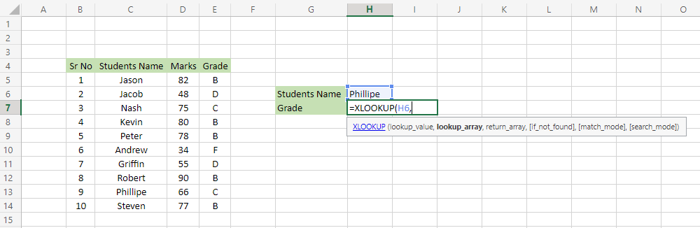
Step 2: lookup_array
Now comes the lookup_array. The lookup_array is the range of cells we need to find our lookup_value. In this case, it is column C consisting of range C5:C14.
Step 3: return_array
The third argument is selecting the range of cells you need to return the value. Any cell corresponding to the lookup_value will be returned from the lookup_array.
An essential difference between the VLOOKUP and our function is that you don't need to select the entire table to look for the values you need to return based on the lookup_value.
All you need to do is select the row or column from which you want to return the result.
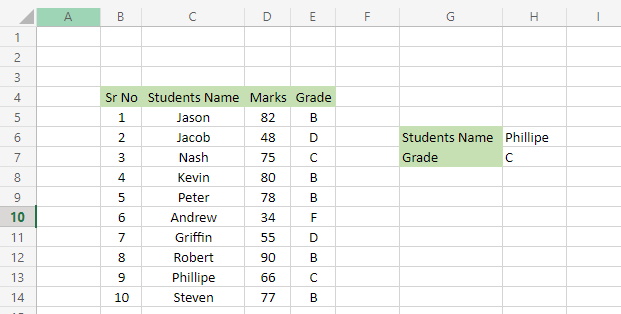
As you can see, we still get the correct result even after using the first three parameters in our formula as
=XLOOKUP(H6, C5:C14, E5:E14)
Step 4: if_not_found
Let's say we use 'Ryan' as the lookup_value in cell H6.
If the function finds 'Ryan' in the lookup_array, it will return the value corresponding to it in the return_array. But what if the weight is not found? It will replace the #N/A error in cell H7.
Hence, to avoid this, we will add an optional if_not_found value as "Value is missing" such that our formula becomes
=XLOOKUP(H6, C5:C14, E5:E14, "Value is missing").
The result that you will get is as illustrated below:
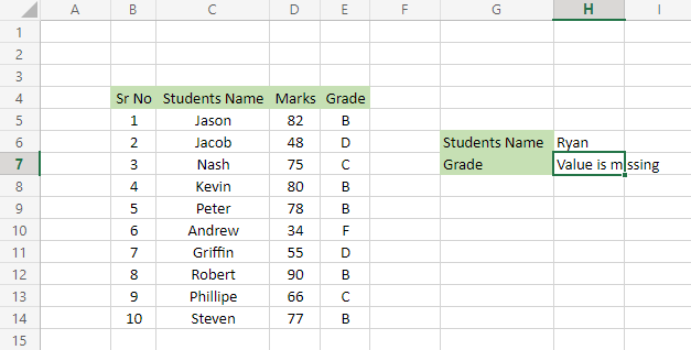
Since 'Ryan' does not exist in the lookup_array, we get an error that has changed to a text value: "Value is missing."
Step 5: match_mode
To see how the match_mode works, we will try to find the next smallest value if a match is not found. Here, we will try to return the marks scored by the serial numbers in column B.
We have updated the data so that all the serial numbers are multiples of two. Using the -1 argument returns the next smallest value, so the formula that we will use is:
=XLOOKUP(H6,B5:B14,D5:D14, "Value is missing", -1).
Now, if the look_up value is 6 or 10, the function works fine and returns the marks.
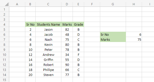
But what happens when you use 15 as the lookup_value? Since the value is not matching, Excel finds the next smallest value in the lookup_array and returns its corresponding value.
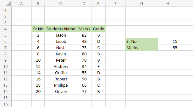
So, for a lookup_value of 15, we got the result for 14, whose corresponding value in the range D5:D14 is 55 marks.
Step 6: search_mode
The final parameter is usually helpful when you need to return the latest value for a recurring lookup_value from the table.
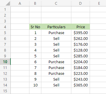
Assume that you wrote journal entries in Excel for all the purchases and sales that you make each day.
The spreadsheet looks as illustrated below:
Here, if you need to find the first or last selling price, you can use 1 or -1 respectively to search from top to bottom or vice versa.
So, to find the earliest "Sell" price, the formula becomes:
=XLOOKUP(G6,C5:C14,D5:D14, “Value is missing”, 0, -1)
This will give you the result as illustrated below:
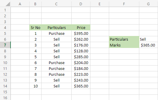
Since $365.00 is the first value from the bottom of the return_array, we get it as our result in cell G7. Similarly, you can use this formula:
=XLOOKUP(G6,C5:C14,D5:D14, "Value is missing", 0, 1)
This will gives the result as $262.00, as it is the first value that matches from the top.
Examples of XLOOKUP function
XLOOKUP is fun when you are making practical implementations on a dataset rather than just reading what you can do with it. Below are some examples where you can use the function to enhance your productivity at work.
Example #1: Wildcard match
The function allows you to make partial matches by using the argument for match_mode as 2. The most used wildcard characters are the asterisk (*) and the question mark(?).
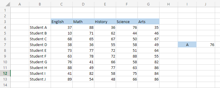
Here, we will return our partial match result using the asterisk as our wildcard character. For example, assume that you have the marks scored by students in different subjects.
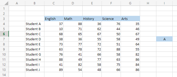
If you need to find the marks scored by 'A' in Science, you will be using the formula:
=XLOOKUP(“*”&I7,B4:B13,F4:F13, , 2)
This will give you the result in cell J7 as:
Notice that we have skipped the optional argument if_not_found in the formula as we did not need an alternative value. Hence, you can miss the deals by keeping the argument empty and moving on to the following idea in the formula.
Example #2: Left lookup
Even though VLOOKUP will be a knight in shining armor for every Excel user, the same armor makes it rigid for the function to be used in different scenarios. Unfortunately, the left lookup is where VLOOKUP fell short of its capabilities.
Excel users adopted a combination of the INDEX and MATCH functions so they could use left lookup but using INDEX MATCH isn't as easy as VLOOKUP and requires a bit of practice.
Years later, a new sheriff in town can do it all - left lookups, conditional searches, and whatnot, you name it! It's none other than the function on which the article is based.
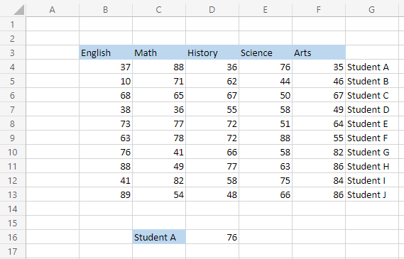
Suppose that your data looks as illustrated below, and you need to find the marks scored by Student A in his Science exams.
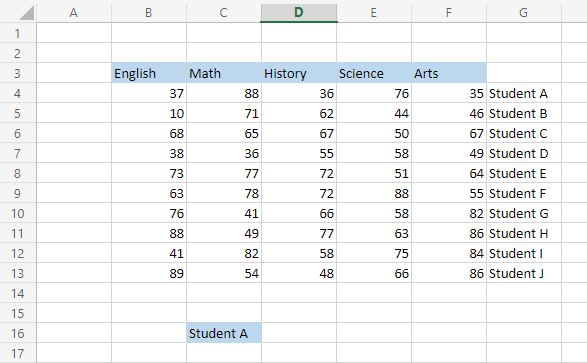
The formula you will use is:
=XLOOKUP(C16, G4:G13, E4:E13)
Our return_array is on the left of the lookup_array. You should get the result:
How simple was that! Just three easy arguments, and you get the result. Since this function is currently only on Excel 365, you can also check out the INDEX MATCH article where we have elaborated on using the INDEX MATCH function in different situations.
Example #3: Getting the last occurrence
We saw how you could get the first or previous occurrence value by changing the search_mode argument. To find the last occurrence of a recurring value, we use the search_mode parameter value as -1.
Suppose that the bank that you work at needs to find out what the last sell transaction amount was from the given data:
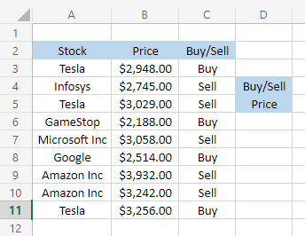
This can be achieved using the formula:
=XLOOKUP(E4,C3:C11,A3:A11,,0,-1)
In cell E5, you will get the result:
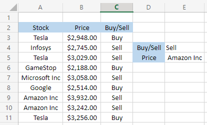
As our lookup_value in cell E4 is 'Sell,' Excel finds the first value fulfilling the Sell criteria from bottom to top and returns the result as 'Amazon Inc,' which corresponds to our criteria value.
Example #4: Return multiple rows or columns
VLOOKUP will only return a value from one row or column based on the col_index_num you input into the formula. However, the procedure references the entire table but only returns values from a single column or row.
On the other hand, by using the XLOOKUP function, you can return values from multiple rows or columns. How would you do that? Instead of referencing a single column as the argument for return_array, you can reference various rows or columns.
For example, if you need to return all the marks for student A, you can use the formula:
=XLOOKUP(C16, A4:A13, B4:F13)
This will give you the following result:
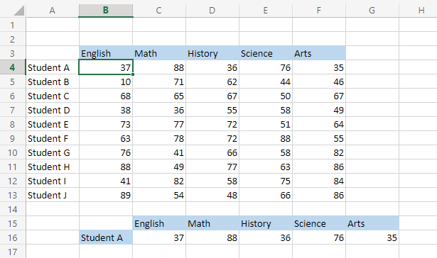
Even though we only use the formula in cell C16, the result 'spills' into the other cells, up to cell G16. Quite a practical approach to avoiding multiple VLOOKUPs.
Example #5: Two-way lookup
Two-way lookups are performed when you want to pull data from any particular cell from the spreadsheet. In simple terms, it's the intersection point of the two nested XLOOKUP functions in the formula.
Here, our first function will use the subject name as the lookup_value, while the second function will use the student name as the lookup_value.
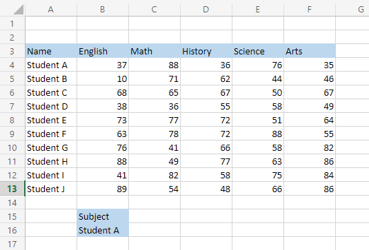
Assume that if you need to find the marks scored by student A in English, the formula that you will use is:
=XLOOKUP(C15,B3:F3,XLOOKUP(B16,A4:A13,B4:F13))
This will give us the result:
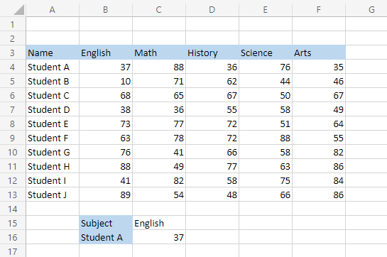
Here, both the cells C15 and B16 are referenced with the values from range B3:F3 and A4:A13, respectively.
How are two-way lookups different? Well, try changing either value in C15 or B16. For example, if you change the subject to 'History' and keep the B16 value as 'Student A,' you will get the result 36.
On the other hand, if you keep the subject as 'History' and change the B16 cell value to 'Student J,' the result automatically changes to 48.
Example #6: Finding a value in multiple ranges
There might be instances where you need to find a particular value in two different tables. In such cases, using nested functions can be extremely useful.
The logic behind using two nested functions is that if the first table cannot return the result, there might be a value in the second table. Therefore, the most crucial factor to consider is the if_not_found argument of the function, where we will use our second XLOOKUP.
So, we are asking Excel to: "If you can't return the value from the first table, search the same value in another table." You can keep doing this nested look up to Excel's limit!
For example, assume that you have two tables below in different spreadsheets for students who have scored marks in their examinations.
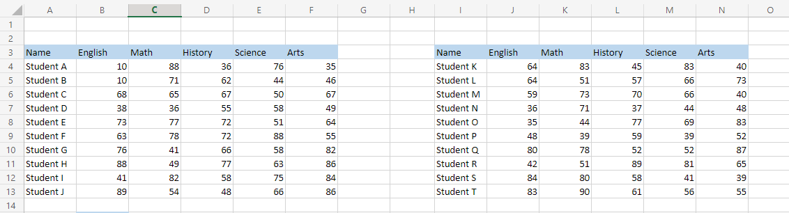
Suppose you need to find the marks scored by Student Q in his English examination, but you are not sure which table has the effects for Student Q.
Here, you will use the following formula:
= XLOOKUP(H15,A4:A13,B4:B13,XLOOKUP(H15,I4:I13,J4:J13)
This will give you the result in cell H16:
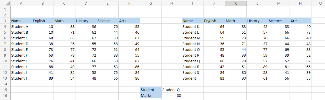
On closer inspection, we find that, since Excel could not return the result from the first table, a second function runs in place of the if_not_found argument and returns the result as 80.
Example #7: Conditional lookup
Even though XLOOKUP is already overpowered with its basic functional features, there is still a feature of conditional lookup that we have overlooked.
By including other functions such as MIN or MAX, you can find which student scored the lowest marks in a particular subject or which student scored the highest.
Assume that you have the data as illustrated below:
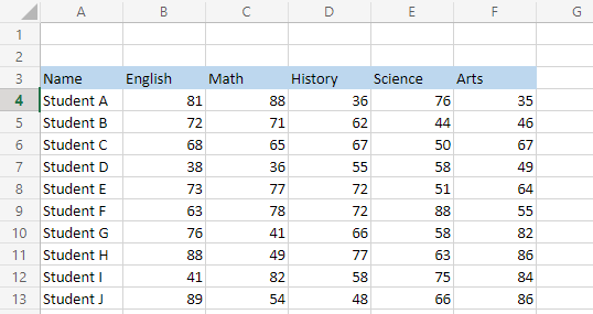
The formula that you will be using to find the student who scored the highest marks in each subject is:
=XLOOKUP(MAX(XLOOKUP(B15,$B$3:$F$3,$B$4:$F$13)),XLOOKUP(B15,$B$3:$F$3,$B$4:$F$13),$A$4:$A$13)
To find the student who scored the lowest marks, use the formula.
=XLOOKUP(MIN(XLOOKUP(B15,$B$3:$F$3,$B$4:$F$13)),XLOOKUP(B15,$B$3:$F$3,$B$4:$F$13),$A$4:$A$13).
For both the formulas, you will get the result:
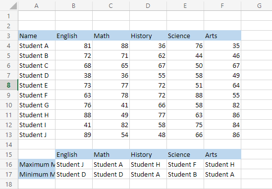
Breaking down the formula, we understand that the first nested function finds the maximum marks scored by the student in that particular subject. Once the maximum effects are returned, it uses the lookup_value in the second nested XLOOKUP that acts as the lookup_array.
Here, our lookup_value will match within the lookup_array, while, finally, the third and final outer function returns the value from the return_array, which is the range A4:A13.
XLOOKUP benefits
There are numerous advantages to using the XLOOKUP over the other lookup family functions, such as VLOOKUP, HLOOKUP, or INDEX MATCH.
1. Straightforward and less error-prone
Since the syntax is quite simple to understand and can be used as a substitute for both VLOOKUP and HLOOKUP, there are hardly any chances of making any errors.
JP Morgan was hit with a $6 million loss due to fundamental excel flaws that resulted from a manual copy and paste of data into different spreadsheets.
As such errors can cause a significant dent in the balance sheet of financial organizations that make widespread use of Excel, formulas that prevent errors in Excel is of the utmost importance.
2. Find the exact match by default
When you use the VLOOKUP, you must compulsorily use the FALSE criteria to find the precise match for the value. However, on the other hand, XLOOKUP finds the exact match for the weight for default.
So, even if someone is not well acquainted with the function and accidentally uses it in their spreadsheet, they can stay assured that the result they will get is correct.
3. Value was not found as a replacement
The problem with using VLOOKUP, HLOOKUP, or INDEX MATCH is that if the weight is not found, excel returns the result as an #N/A error.
Then, it would help if you used the IFERROR function to replace the error with another value. This improved function, however, comes equipped with the value_not_found argument by default.
It is an optional feature where you can input the value you need in case Excel cannot find a match for the corresponding value.
4. Look for the value starting from the bottom or top
The search_mode argument allows you to either look for the value from the bottom to the top of the lookup_array or in the inverse direction, i.e., from top to bottom.
5. Faster results
VLOOKUP can slow down your spreadsheet since you are referencing a large amount of data in the formula. As a result, it takes far more processing time to give you the final result when there are hundreds or thousands of rows.
On the other hand, when using XLOOKUP you are only referencing the column or row from which you need to return the result. Therefore, the processing is much quicker than VLOOKUP.


or Want to Sign up with your social account?