REPLACE Function

What is the REPLACE Function?

REPLACE function is an Excel function that falls under the category of String/Text functions. It replaces a set of characters in a string with a different set of supplied characters based on the location. 

For example, you can change the file’s path using the replace function such that D:\Excel_Practice_Files\Practice_File_1.xlsx becomes E:\Excel_Practice_Files\Completed\Practice_File_1.xlsx. 

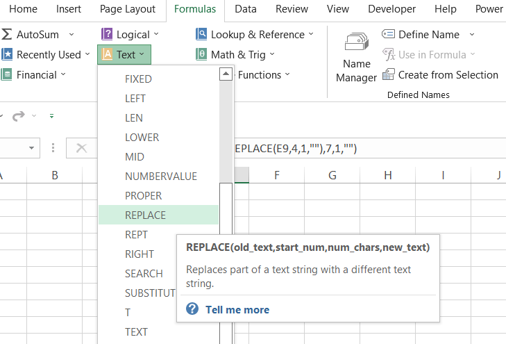
It is usually helpful while creating macros that save the completed file in a separate folder once it completes the task. In the Formulas tab, you can find the function in the ‘Text’ function library. Additionally, you can also use it as a part of the formula in the Excel spreadsheet.

REPLACE Function Formula

The syntax for the replace function is :

=REPLACE(old_text, start_num, num_chars, new_text)

where,

• old_text = Original text from which we want to replace some characters. This is a required parameter
• start_num = The character’s starting position in old_text that you want to replace with new_text. This is a required parameter
• num_chars = The number of characters that will be replaced from the old_text by the new_text. This is a required parameter
• new_text = The text that is supplied to replace the characters from the old_text. This is a required parameter

How to use the REPLACE Function in Excel?

Suppose that your organization’s employee portal system generates the employee information in an Excel spreadsheet in the following manner:

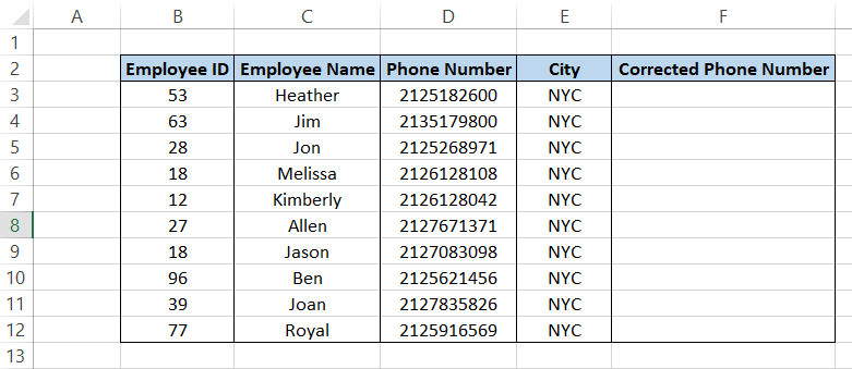
However, due to specific requirements, you need the phone numbers in proper format with a dash (-) between them such that the value in D3 becomes 212-518-2600. For this, we will be using a nested REPLACE such that our formula becomes =REPLACE((REPLACE(D3, 4, 0, “-”)), 8, 0, “-”).

If we break down the formula into two separate entities, our nested formula becomes REPLACE(D3, 4, 0,”-”). Here our old_text argument is the referenced D3 cell while the starting position to replace characters is 4.

Since we use 0 as the number of characters to replace, the function adds up our new_text value in the original text. So we get the result as 212-5182600. However, that’s not the required format which we need for the phone numbers.

So we use an additional REPLACE on the outer side with the nested REPLACE(D3, 4, 0,”-”) as our old_text.

Now you need to count the characters as per the result for the nested if or else you will get the wrong result if you count the characters directly from cell D3. Thus the final formula becomes  =REPLACE((REPLACE(D3, 4, 0, "-")), 8, 0, "-"). This will give you the result as 212-518-2600 in cell F3.

When you drag down the formula, the spreadsheet will look as below:

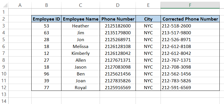
Remember that REPLACE works excellent based on locations. So if you have data where the data integrity is constant such as phone numbers or file locations in computers, it is a great asset to use. 

The only limitation to the formula is that you can’t usually drag it down to accommodate other values in function if they don’t have the same format. For example, assume that you have the below data:

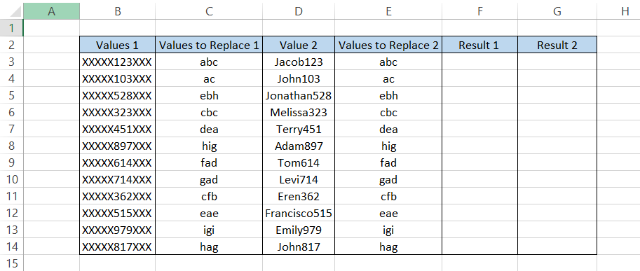
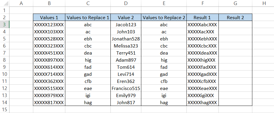
As you can see, the values in column B all have a consistent format starting with XXXXX(five X’s) followed by numeric digits and then again XXX(three X’s). The values that will replace the numeric digits in column B are present in column C.

When we use the formula =REPLACE(B3, 6, 3, C3) in cell F3, we get the result as XXXXXabcXXX. Since the format is constant, we can drag down the formula to get the results as:

But what about the values in the D column? They don’t seem to have a similar format before the numeric values. For example, some values in the D column may have 5 characters before the numeric value, while some may have 7 characters.

As a result, we usually can’t drag the formula =REPLACE(D3, 6, 3, E3) until the cell G14 as you may get deviating results.

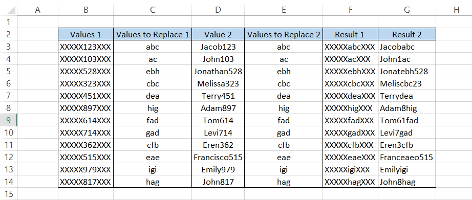
Here, it would be best if you manually assigned different starting positions to the text with which the new_text would be replaced. For example, the starting position for the formula used in cell G4 will be 5 as opposed to start_num, which was 6 for the formula used in cell C3.

So does that mean that manually assigning a different starting position is the only way we can get the desired result in column G? Absolutely not! 

Another way you can use to get the desired result is by using the combination of LEFT, LEN, and REPLACE . This might get a bit complicated but try to keep up with us. You will need to make two additional columns.

In column H, we will be using the formula =(LEFT(D3, LEN(D3) - 3)), which basically takes the string in cell D3(Jacob123) and returns a string from the left with n number of characters less than the string. 

The LEN function gives the length of the string, which in this case is 8. So the final formula provides us with the result as Jacob. The formula LEN(D3) - 3 is dynamic so that for the next value, it will get the total length of the string and then subtract three from it to return the result.

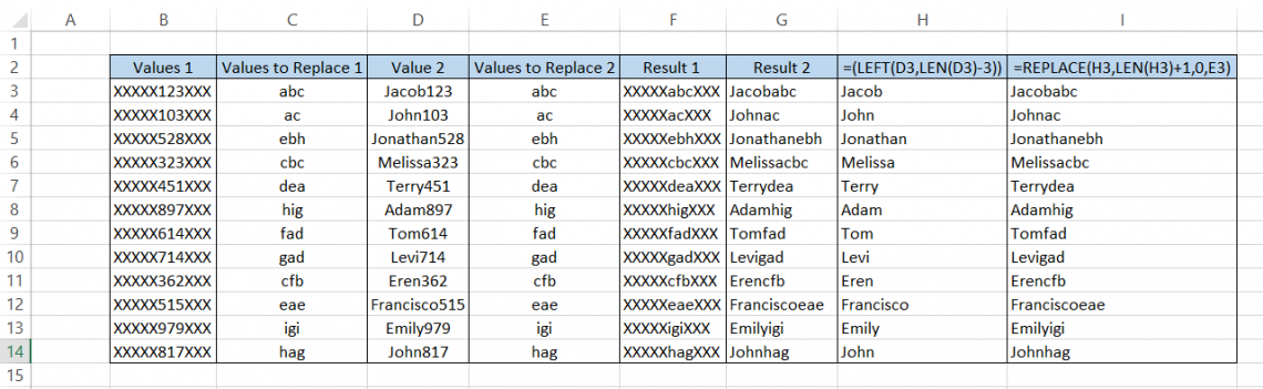
When you drag the formula down, you will get the result as:

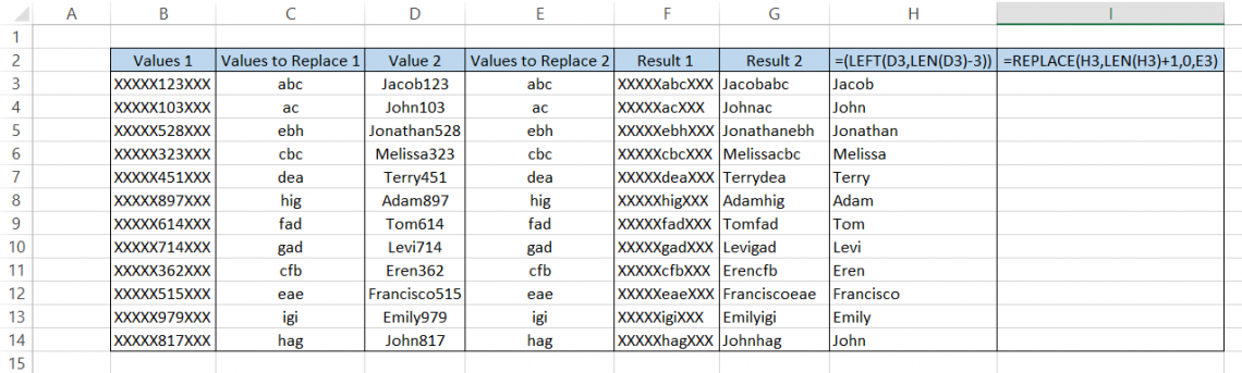
This completes the first part of the final expected result. Next, we use the formula =REPLACE(H3, LEN(H3) + 1, 0, E3) where we reference the value from column H, use the start_num parameter as the value in column H itself (since we are expecting the values to concatenate in the end). 

The difference here is the addition of 1 to the LEN(H3) function, which, if not followed, will not give the correct result, i.e., it will replace the last character of the strings. Finally, after you drag the formula up to cell I14, you will get the same result as column F.

We know how smart Excel is at doing any task, or to better frame it, it can perform the same task in different ways. 

SUBSTITUTE function

Another way you can correctly replace the numeric values by the values in column E is by using the SUBSTITUTE function and the RIGHT function.The formula that we will be using is =SUBSTITUTE(D3, RIGHT(D3, 3), E3, 1), which gives us the correct result in the spreadsheet as illustrated below:

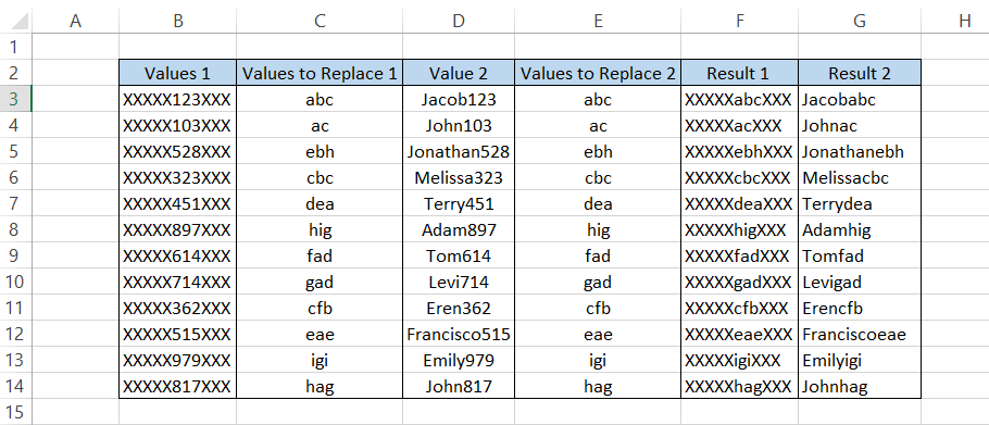
By breaking down the formula, we understand that the RIGHT function captures the first three characters from the right side of the string, i.e., 123, and the SUBSTITUTE function replaces it with the value in cell E3 to give us the final value in cell G3 as Jacobabc.

Finally, if we drag down the formula up to cell C14, we get the text that contains characters replaced with numeric values. We will see more on the SUBSTITUTE function in the following few sections.

REPLACE vs. SUBSTITUTE function

SUBSTITUTE function is another function that falls under the category of String/Text function. It replaces a set of characters in a string with a different set of characters.

Thus, if you want to replace a specific text in a string based on a predefined search, such as changing ‘dog’ to ‘cat’, you should use the SUBSTITUTE function. 

On the other hand, if you need to replace any text in general based on position, then the function that will work best is the REPLACE function.

The syntax for the SUBSTITUTE function is:

=SUBSTITUTE (text,old_text,new_text,[nstance])

where,

• text = Original text from which we want to replace some characters. This is a required parameter
• old_text = characters from the text string that are replaced. This is a required parameter
• new_ text = characters that we will replace the old_text with. This is a required parameter
• instance = the index number of the nth recurring old_text that you wish to replace the new_text with. This is an optional parameter which, if not specified, every occurrence of old_text is replaced by the new_text

How to use the SUBSTITUTE function in Excel?

The SUBSTITUTE function works excellently in data cleansing tasks such as the irregular format for phone numbers. For example, suppose that you have the following data with phone numbers that are not standardized:

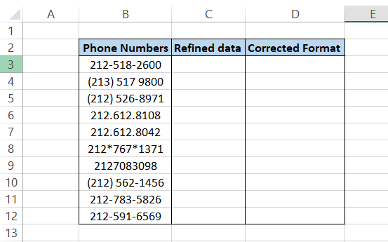
As you can see, the phone numbers are in several different formats. Therefore, such irregularities can affect the integrity of the data if you make a macro that identifies a particular format such as XXX-XXX-XXXX. 

Hence, you can use the SUBSTITUTE function to refine the data by removing all the symbols that occur in the phone numbers. The formula that you will be using to first get a more ‘cleaner’ data is

=SUBSTITUTE(SUBSTITUTE(SUBSTITUTE(SUBSTITUTE(SUBSTITUTE(SUBSTITUTE(B3, "-", ""), "(", ""), ")", ""), " ", ""), "*", ""), ".", "")

Don’t freak out! The formula looks very complicated and lengthy, but on closer look, it’s just repeating the same thing over and over, similar to a loop. The result you will get using the formula in column C is:

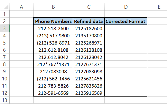
Now our data has some uniformity in its format after removing all the symbols. After breaking down the formula, we see that the substitute function merely replaces the symbols such as dashes (-), brackets, dots (.), and asterisks (*) with empty strings.

Since the functions are nested, it keeps removing those symbols until there are only numbers in the cell value. For example, the formula SUBSTITUTE(B3, ”-”, ””) in cell D5 will give us a result of (212) 5182600.

There are still three different characters, i.e., brackets and spaces, that need to be removed to have a uniform format for the phone number. So again, you will use the formula SUBSTITUTE, but this time the earlier formula will be nested inside this function.

The formula will become SUBSTITUTE(SUBSTITUTE(B3, ”-”, ””), ”(“, ””) which will give you the result as 212) 5182600. That's how we arrive at our final formula, which gives us the values in column C.

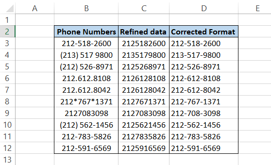
The final step is to give the corrected format in column D. We will be using the REPLACE function such that our formula will be =REPLACE(REPLACE(C3, 4, 0, "-"), 8, 0, "-").

We don't replace any characters by using zero as our num_chars parameter but add an additional character in the form of dash (-). This is done twice using the nested formula. The final result in column D will be as follows:

More on Excel

To continue your journey towards becoming an Excel wizard, check out these additional helpful WSO resources.

• Excel keyboard shortcuts for Windows and Mac
• Advanced Excel formulas you must know
• Best Excel courses
• Developer tab
• How to Group in Excel