Slicer in Excel
Maximize your pivot tool usage through a slicer in Excel.


What Is A Slicer in Excel?
In Excel, Slicers enable you to filter your dataset when you click one or more buttons on the slicer’s interface. They behave as visual filters for your data (including pivot charts & pivot tables) which can be used by clicking on the buttons corresponding to different rows/column headers.
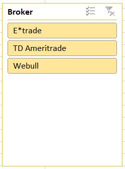
The yellow-colored boxes are the slicers in the above example. This article will guide you on how you can add this excellent feature to your dataset as well!
- Slicers in Excel are powerful visual filters that allow users to interactively filter data in pivot tables and charts by clicking buttons corresponding to different categories or dimensions.
- Adding slicers to pivot tables enhances data analysis and visualization by providing a user-friendly interface to dynamically filter data based on various criteria such as brokers, portfolios, or product categories.
- Customizing slicers in Excel enables users to adjust their appearance, color, size, and layout to match the aesthetics and requirements of their spreadsheet or dashboard.
- Slicers can be linked to multiple pivot tables or charts, facilitating cross-filtering and creating interactive reports that dynamically update based on user selections, enhancing data exploration and decision-making processes.
How To Insert Slicer To Your Regular Excel Pivot Table?
Suppose you have the following hypothetical data set spanning thousands of rows below.
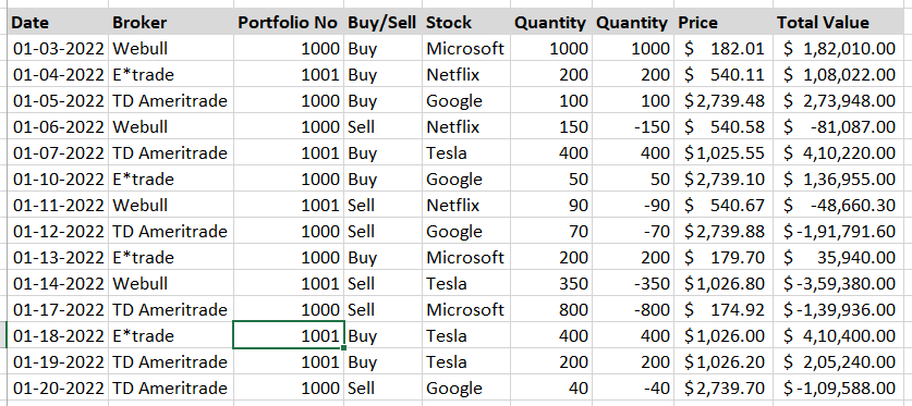
A pivot table is created that shows the summary of Buy/Sell transactions for stocks in each portfolio using different types of brokers.
Our final summary table looks as below:
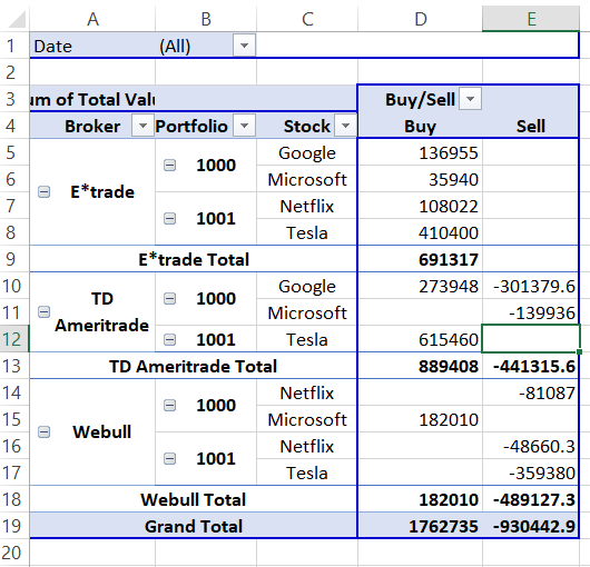
Since our pivot table is now prepared, we can add the slicers to our dataset. So now, if you want to filter your data, let’s say by broker or portfolio number, you can do this in two different ways.
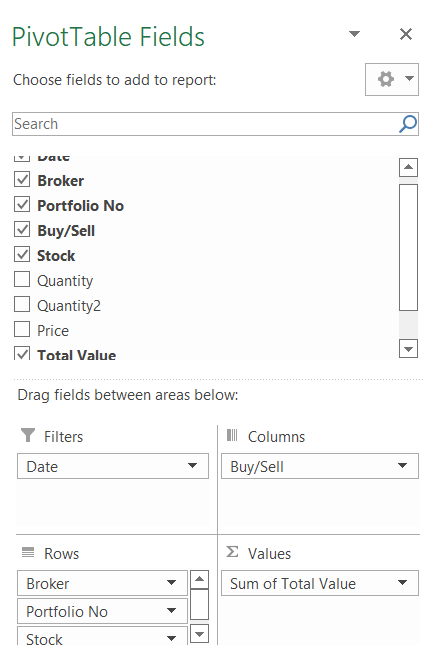
- Add broker as a filter for your report in pivot table fields
- Add a slicer for the broker and click on the required buttons that you want.
As we have already covered how filters work in the pivot table guide, we will focus on inserting slicers and how they work in this article.
- Select any cell of the pivot table.
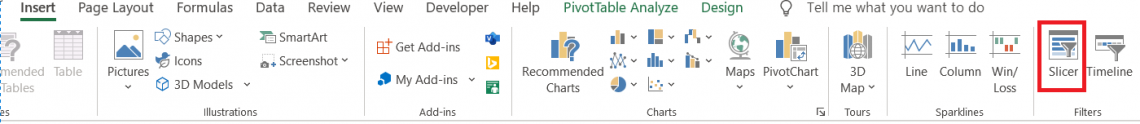
- Click on the Insert tab and navigate to the Filters section. This is where you will find the Slicers. Click on it.
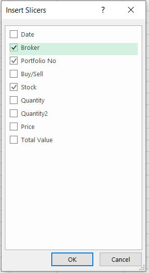
- This opens the Insert Slicer dialog box, where you need to select headers for which you need to create filters. You can choose more than one dimension from all the available dimensions in the dialog box. For example, let’s say we select the dimension as a broker. Click on OK.
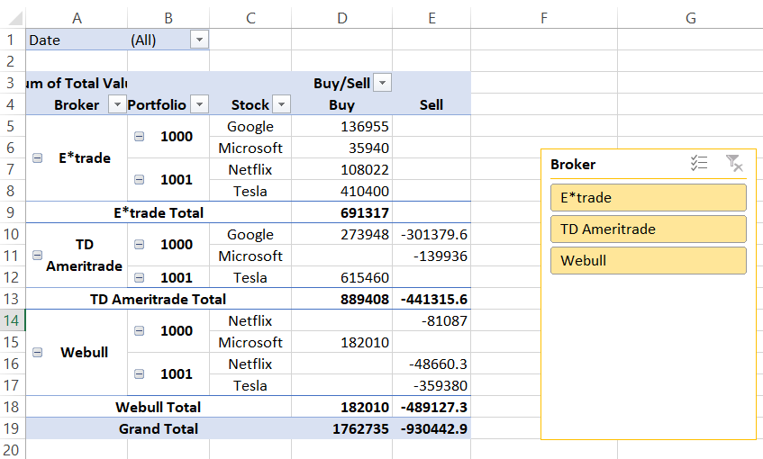
Similar to pivot tables, where the table identifies unique items in its row and column-oriented perspective, Slicers list down all the dimensions only once in its box. So this is how your pivot table will look like along with the slicer:
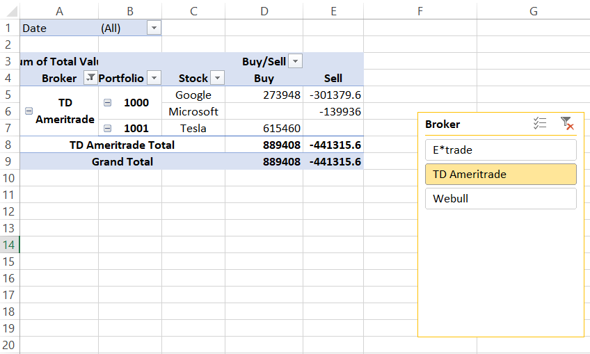
Now try clicking on one of the buttons in the broker slicer, let’s say TD Ameritrade. You will see that the slicer filters the data so that the buy/sell transactions exist in the portfolio only for TD Ameritrade. Amazing Right?!
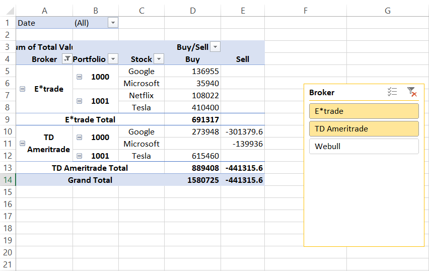
If you wish to choose multiple dimensions simultaneously, simply hold the Ctrl key and click on the buttons that you want your pivot table to display. For example, we have selected E*trade and TD Ameritrade in our slicer to give our summary table as:
If your table consists of a more extensive set of dimensions and you need to clear your entire selections, you can click on the filter icon at the top right of the slicer. This icon will be represented with a red cross, indicating that it removes the filter from our dataset.

Formatting Slicers
Once you insert the slicers, you can customize them as per your requirements. This includes the appearance, color, caption, alignment, etc. For example, if you need to change the color of the slicer:
- Select the slicer. Click on the Slicer tab in the list of tabs.
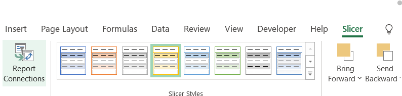
- Navigate to the Slicer Styles section, where you can change the color of the slicer.
- If you have a large number of items in your slicer, you can also change the height and width of the slicer, along with the option to increase the number of columns.
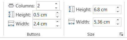
- Click on the Slicer tab, where you will find the buttons section that allows you to change the height & width of the buttons on the slicer while the size sections change the overall dimensions of the slicer. The default column in slicer is one, but for our dataset, we have added two columns, as shown below:
Using Multiple Slicers
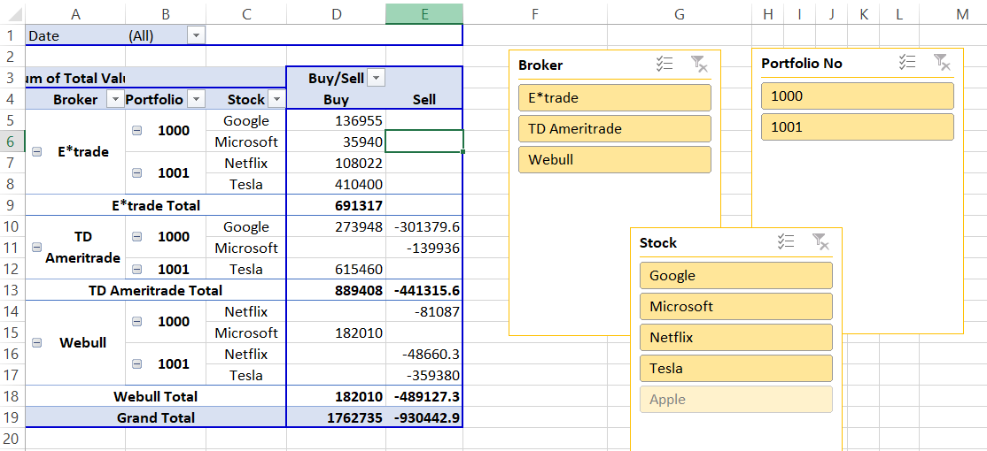
You can use multiple slicers by selecting more than one dimension from the Insert slicer dialog box. For example, we have chosen the broker, stock, and portfolio number as our three different slicers.
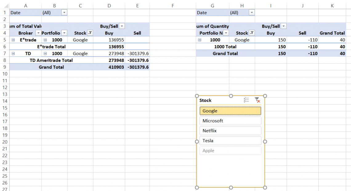
Next, click on OK. This is what your spreadsheet will look like:
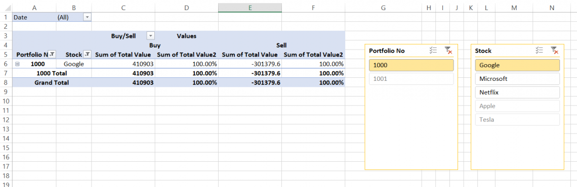
Now, if you want to check, what was the buy/sell transaction amount for Google in Portfolio 1000 using E*trade as your broker, all you need to do is click on the respective buttons.
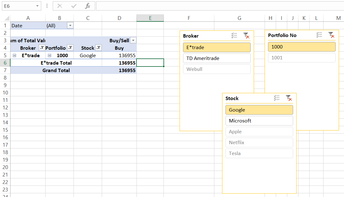
We see that only buy transactions amounting to $1,36,955 were made for Google stock in Portfolio 1000 using the E*trade broker. By holding the Ctrl button & making multiple selections, we can build customized filter pivot tables.
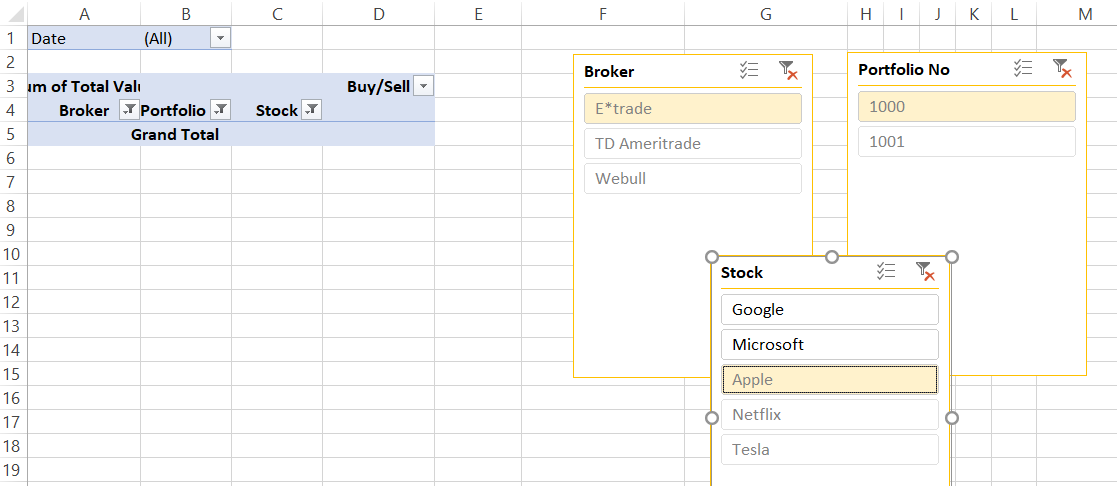
Notice that some of the buttons in the slicer are translucent? This means that we do not have any data for the respective fields in our pivot table.
If the button appears light-colored when selected, it means that the data does not exist for it, as indicated by our summary table.
Interactive charts using Slicers
Assume that you have the pivot data for prices of movie tickets for teenagers, adults, and senior citizens (above 65 years of age), respectively. Our dataset for the ticket pricing is as below:
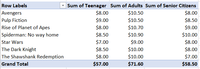
Now, let’s say you need a chart comparing the ticket prices for the mentioned age groups. You can do this by creating interactive charts with the help of slicers.
- Once your pivot data is set up, add a slicer which, in this case, we have selected the movie name.
- Now create a pivot or regular chart by clicking on the Insert tab and navigating to the charts section to select the desired chart type (e.g., Clustered column chart)
- After formatting, your interactive charts are ready to be put to use.

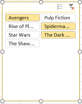
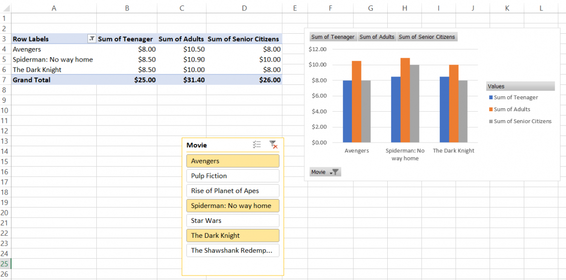
Let’s say you need to compare the price of three different movies - Spiderman: No Way Home, Avengers & The Dark Knight. Hold the Ctrl key and click on the three movie buttons. You will see that your chart and the pivot table start to change in their structure.
This is how your charts, as well as the pivot table, will look like:

Slicer linked to multiple pivot tables
Another advantage of using slicers is that you can build cross-linked reports connecting each other. This means building two separate pivot tables and building a connection between them (that’s literally the function’s name) to give you the final interactive reports.
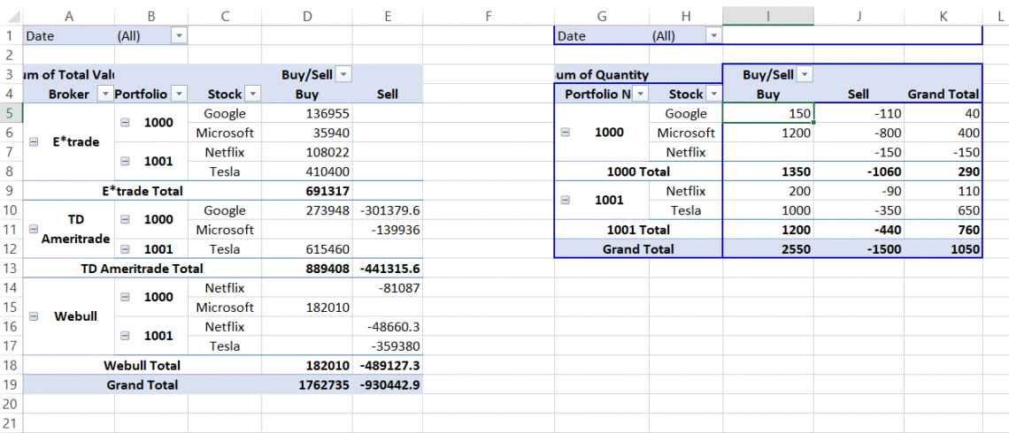
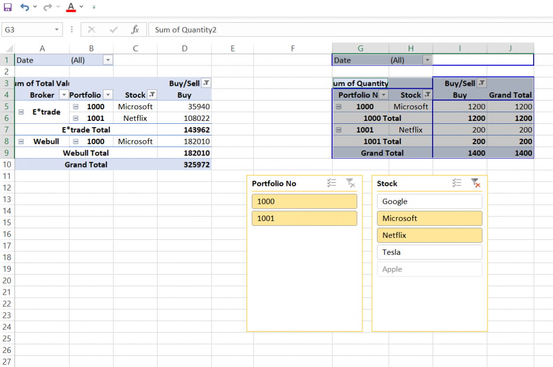
Assume that you build two different summary tables as below, where one displays the quantity of bought/sold stocks while the other shows the total value of buy/sell transactions (you can add them on the same sheet by selecting Existing Sheet as your preference for inserting pivot table).
The next step is to add slicers.
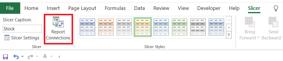
- We have inserted a slicer for the field Stock in our spreadsheet. To build a connection between the pivot tables, go to the Slicer tab, and click on Report Connections in the Slicer section.
- This will open the dialog box where you can select the pivot table you want to establish the connection. You can connect pivot charts, too, using Report Connections.
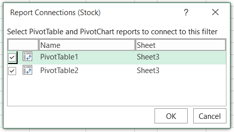
- Click on OK. Now select options in the slicer menu, like Google, and it will automatically filter both the tables.
- Similarly, you can add multiple slicers to cross-link two or more pivot tables in your dataset. However, you need to establish connections for each slicer to the pivot table individually, which can be quite a drag if your dataset is extremely large.
- You can also build cross-linked pivot tables by cross-linking two tables. This makes our charts more robust and interactive.
Note
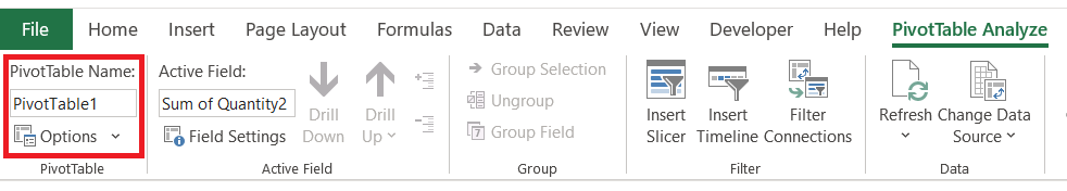
It is always good practice to name your tables and charts before establishing the connection. Then, if you have multiple tables in your spreadsheet, you can correctly link the tables and avoid mistakes that can break your spreadsheet models.
Slicers along with formulas
You can make slicers to interact with the formulas in your spreadsheet. A dummy pivot table is the easiest method to capture the slicer selection into your cell. Let’s explore this concept with an example so you can get a better grasp of it.
Suppose that you run a restaurant called WallStreet Cafe and Burgers.
Since the initial investment was quite high, you need to get your restaurant running, or else your main competitor MrBeast Burgers, a fast food outlet run by teen YouTubers (all information in this example is fictitious and is not based on real people), might just close down your restaurant even before it begins.
Now all you need is billing software for your outlet. So you place a freelancing job on Fiverr, and the guy (Adam in this case) builds you a spreadsheet model for $25 that takes care of the billing.
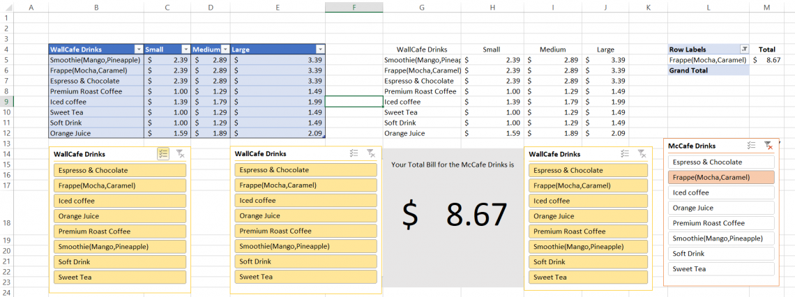
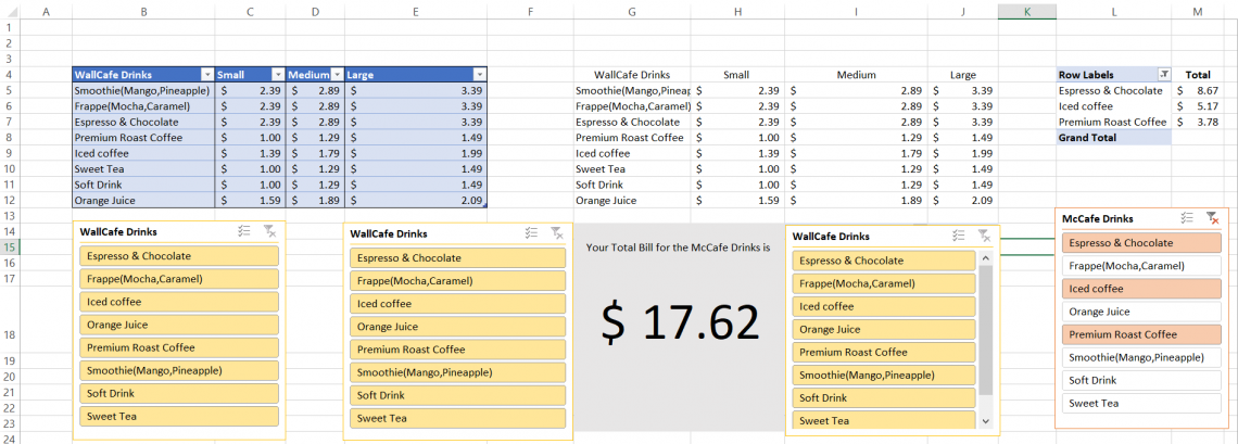
This is how the spreadsheet looks:
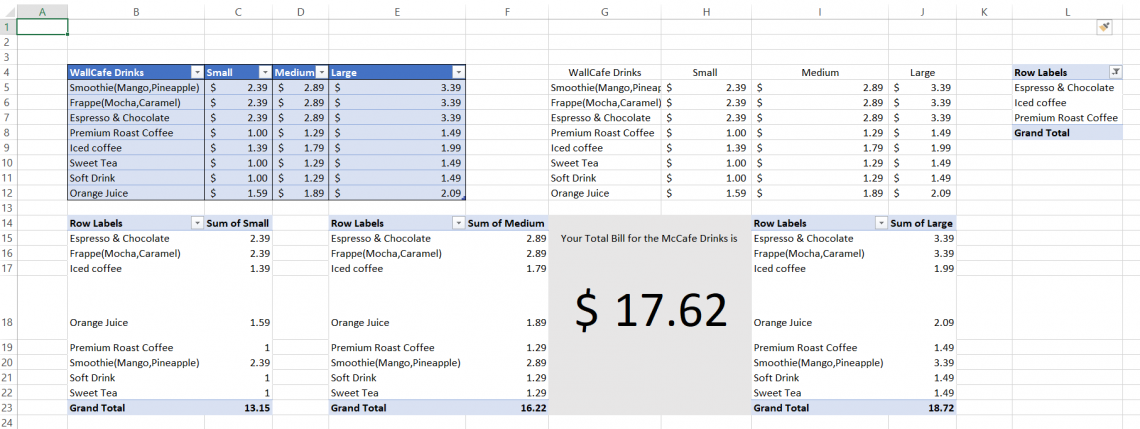
So the first order comes for the day, whose summary is as below:
You select the order on your billing system, and it shows the total amount as:
A flawed system but still good to get your business running, right? Let’s see how the spreadsheet works to understand better how the dummy pivots work along with the formulas.
Firstly the Excel sheet consists of the menu in the range B4:E12.
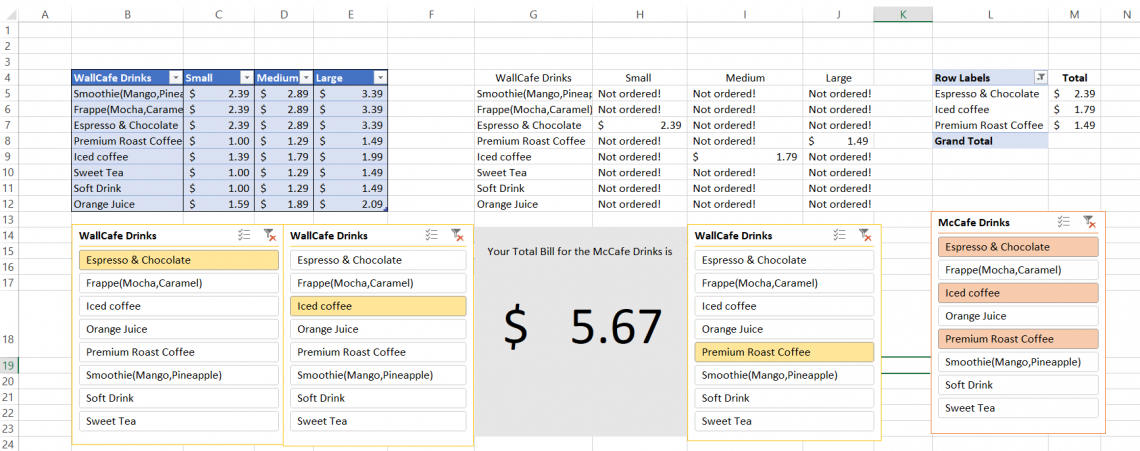
Based on it, Adam creates a dummy pivot table for the field ‘WallCafe Drinks’ in a row-oriented perspective in cell L4. Next, he creates pivot tables that display the drinks and the price for the different sized drinks, i.e., small, medium, and large, respectively.
These three pivot tables work as an ordering system, while the dummy pivot in cell L4 works as a billing system. The table in range G4:J12 will work as your order summary screen to show what the customers have ordered.
Since most customers won’t order all the items on the menu, slicers will be needed to filter out your menu (We will assume that most customers order at least one item from all the different sized drinks, i.e., small, medium, and large.
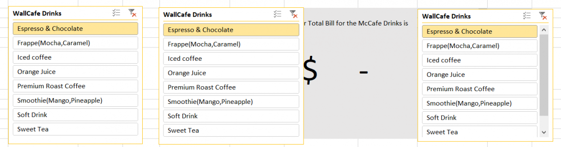
Four similar types of slicers are added for the dimension’ WallCafe Drinks’ and report a connection such that every slicer filters a separate pivot table.
For example, a slicer that filters the amount for small-sized drinks and so on. Then, Adam places those visual filters onto the pivots to ‘hide’ them to make the spreadsheet billing system more appealing.
This completes the formation of the spreadsheet model in terms of physical appearance as below:
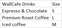
The critical part is the formulas that display the order summary table and the total billing amount. For this, Adam uses the formula =IFERROR(VLOOKUP(G5, $B$15:$C$22, 2, FALSE), “Not ordered!”) in cell H4 and drags it down up to H12.
The table array, in this case, is the pivot table that Adam had created for the different-sized drinks. So whenever you click on the slicer buttons, let’s say Orange juice, it will display the price for the small-sized OJ.
Similarly, if you hold the Ctrl key and click more than one button, it will display the price in your order summary screen.
Adam copies the same formula in cells I4 and J4 and drags them down while changing the table array for both formulas to the pivot tables in E14 and I14, respectively. This completes the order summary screen.
Next is the billing screen. This comprises our dummy table in cell L4. Since the billing will be based on your order summary table, Adam uses the combination of the Index Match formula =IFERROR(SUM(INDEX($H$5:$J$12, MATCH(L5, $G$5:$G$12, 0), )), “") in the cell M4 and drags it down till M12.
By breaking down the Index Match formula into two parts:
- Firstly he uses the range H5:J12 for his INDEX reference table or the array
- Then he uses the dummy pivot table value as his lookup_value and the column in the range G5:G12 as his lookup_array.
So if the dummy pivot table shows the value ‘Iced coffee’, the Match function will use it to look it up in column G, and the Index function will return the value based on it from columns H, I, and J.
Note
If you are not well versed with the INDEX MATCH function, check our article here to help you master the formula in no time!
Since those are three different columns of the same table referenced, Adam added a SUM function so that we get the total value in the M column (In case, let’s say a customer buys Orange Juice of small, large, and medium-sized each for the same item on the menu)

He then takes the sum of the cells using the AutoSum (more about it here), which is displayed in cell M13.
Note
An important function to use when your formula gives an error is the IFERROR function. If the cell in your spreadsheet shows a #N/A or #VALUE! Error, you can use a nested IFERROR to return a more friendly result. In this spreadsheet, Adam returns the result as empty cells if the customer does not order that item.
So how does the billing spreadsheet work?
Let’s say a customer orders three Espresso and Chocolate small, medium, and large, respectively. Then, you select the buttons for those orders in your ordering table as shown below:
Your manager confirms the order in the order summary table before processing the order. For example, the order summary table looks as follows:
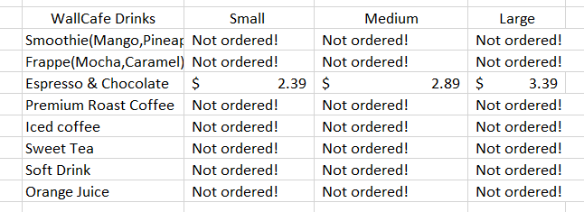
Once confirmed, he then heads over to the billing section of the spreadsheet to generate the bill. Since the order consists of only Espresso & Chocolate, he selects the slicer button for the same.
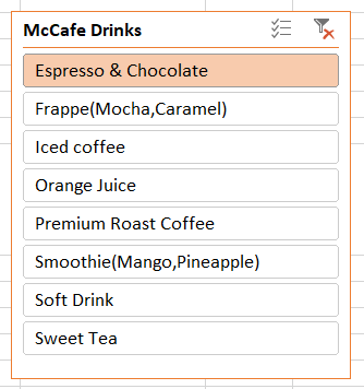
This gives the breakdown of the order in the table placed in L4 and the total.
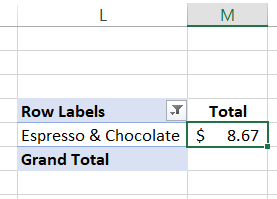
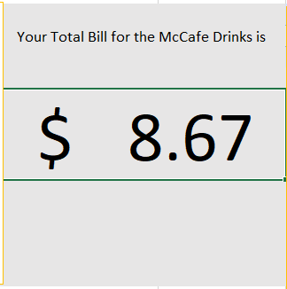
For more than one item in the billing summary section, the grand total in cell M13 is referenced to G18. No matter what the customer orders, after selecting the appropriate buttons, you will get the billing amount in cell G18 which in this case is $8.67.
We hope that this article is helpful for you! If you want to learn more about pivot tables to incorporate the slicers better, check out our article on pivot tables here!
Conclusion
Excel slicers offer a seamless and intuitive way to filter and interact with data in pivot tables and charts, empowering users to gain deeper insights and make informed decisions.
By providing a visual interface for data exploration, slicers enhance the usability and effectiveness of Excel spreadsheets, enabling users to analyze complex datasets with ease.
Furthermore, the ability to customize slicers and link them to multiple pivot tables or charts adds versatility and flexibility to Excel-based data analysis workflows.
Whether creating interactive dashboards or performing detailed financial analysis, leveraging slicers in Excel can significantly streamline the process and enhance the overall effectiveness of data-driven tasks.
More on Excel
To continue your journey towards becoming an Excel wizard, check out these additional helpful WSO resources:


or Want to Sign up with your social account?