CELL Function
An Excel Information function that returns information about the formatting, location, or contents of any cell according to the sheet’s reading order.


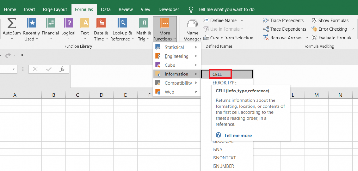
What is the CELL Function?
The CELL function is an Excel Information function that returns information about the formatting, location, or contents of any cell according to the sheet’s reading order.

The CELL function can prove to be particularly useful in extracting specific information about a cell which can be used to users advantage in different situations.
As the name suggests, information functions provide critical information about the cells, spreadsheets, or workbooks.
Unfortunately, they do not get the same level of importance from the Excel community as the Arithmetic or the Lookup functions.
Even if you ask any Excel geek, he would willingly let you know how to use INDEX MATCH or even more complicated formulas. But yes, not the Information functions, or else be ready for an uncomfortable silence.
We at WallStreetOasis are firm believers that everything and everyone has a role to play, whether big or small, in this colossal universe, and the same is the case with the CELL function.
In this article, we will see the CELL function and how it works, along with in-depth examples.
- The CELL function is categorized as an information function that returns details on a particular referenced cell's format, address, column size, row size, etc.
- The CELL function returns information about the formatting, location, or contents of a cell. It's particularly useful when you need to retrieve specific information about a cell for use in formulas, data validation, or conditional formatting.
- The CELL function returns different types of information based on the info_type provided.
- The CELL function is useful for various tasks such as constructing dynamic formulas, extracting data for reports, checking cell formatting, and more.
How the CELL function works?
Earlier, we spoke about the Information function, which makes it obvious what category the CELL function falls under.
The CELL function can return information about the cell address, color, contents, format, etc., based on the referenced cell.
The function has in-built criteria whose information can be found in the Excel file. These are the arguments the function can accept, and anything beyond that will return an error.
The syntax for the function is
=CELL(info_type, [reference])
Where
- info_type - (required) the text value which specifies what information to look for in Excel
- reference - (optional) a connection to a specific cell in the spreadsheet
NOTE
If the reference argument is ignored, the function automatically assumes the information in cell A1.
The different types of text values that you can use for info_type argument are:
| Text Value | Description |
|---|---|
| address | Returns the cell reference as a text string |
| col | Column number of the referenced cell |
| color | Returns the value 1 if the referenced has a negative value and is formatted with a color, or else 0 |
| contents | Replicates the content of a cell if it is a hardcoded value. The result of a formula is returned if the referenced cell has a formula |
| filename | Returns the filename and path where the file is saved as a text string. The function returns an empty string if the file is not saved. |
| format | Returns a code corresponding to the number format of the referenced cell |
| parentheses | Returns the value as 1 if the referenced cell is formatted with parentheses and 0 if not. |
| prefix | Returns a value corresponding to the ‘label prefix’ of the cell. |
| protect | Returns the value as 1 if the cell is locked or else 0 |
| row | The Row number of the referenced cell |
| type | The value corresponds to what type of data is present in the cell. For example, ‘b’ stands for a blank or empty cell, ‘l’ stands for the label(text strings), and ‘v’ stands for the value(all the remaining data types) |
| width | Width of the column |
The information regarding different cells can be obtained only when you use the optional argument reference, or else it will return the result for cell A1.

Example of the Cell function
This section will show how the different text values work to give varied results using the function. The function holds a lot of importance in the VBA codes; however, if you imagine, you may find it has limited functionality.
When you ignore the reference argument in the function, the text values correspond to the first cell, i.e., A1. Only when you include the reference argument can you get a customized result for different cells?
The examples of different values of the function are:
a. address
The ‘address’ argument returns the cell address as a text string. If the reference argument is ignored, then the function returns the address for the first cell. The formula to return the cell address for the first cell is =CELL(“address”), which gives the result as A1.
Similarly, to return the cell address for B5 in cell B2 as a text string, we will use the formula =CELL("address",B5), which gives the result:
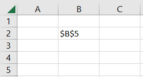
The cell address represented as a text string would change every time a different reference is made.
b. col
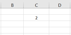
‘col’ returns the column number of the referenced cell. For example, if any of the cells in the second column is referenced in the formula, say =CELL("col",B5), then the function returns the result as 2.
Similarly, suppose a different column is referenced using any cell in the F column. In that case, the formula becomes =CELL("col",F5) to give the result as 6.
c. color
The ‘color’ argument returns the value as 1 if the referenced cell has a negative value plus formatted using a color. If not, then the function returns the result as zero.
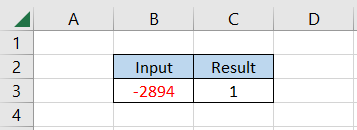
For example, in cell B3, the value is -2894, and the text is highlighted in red font.
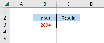
When we use the formula as =CELL(“cell”,B3), we get the result as 1.
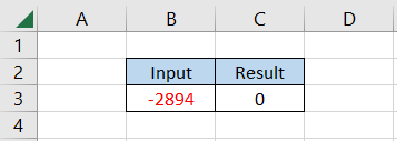
When the formatting is removed, the function returns the result as zero.
d. contents
The function returns the cell contents when you use ‘contents’ as the value. If a formula is used in the cell, the function returns the result, while the exact value is returned if there is a hardcoded value.
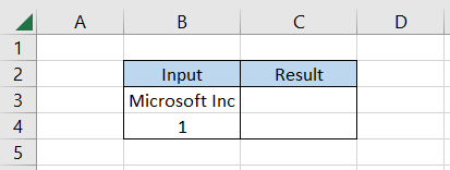
For example, suppose we have the value as ‘Microsoft Inc’ in cell B3, and another is a formula =IF(1>0,1,0) in cell B4, which yields the result as 1.
When we use the formula as =CELL("contents",B3) in cell C3 and drag it down in cell C4, we get the result
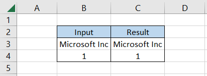
Despite having a formula in cell B4, Excel ignores it and returns the result. In contrast, the hardcoded value is returned as it is.
e. filename
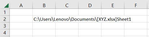
The ‘filename’ is a unique argument that won’t work unless you have already saved the file in the system. Let’s say you open a new file and directly use the formula as =CELL("filename",A1), giving the result an empty cell.
On the other hand, when the file is saved to any name, ‘XYZ,’ and the same formula is used, the result is equal to the entire file path with the file name and the sheet in the end.
f. format
The ‘format’ argument returns a code corresponding to a particular numbering format in Excel.
First, let’s see what different types of code you would usually encounter after using the function, as illustrated below:
| Code | Formatting Description |
|---|---|
| G | General |
| F0 | 0 |
| ,0 | #,##0 |
| F2 | 0 |
| ,2 | #,##0.00 |
| C0 | $#,##0_);($#,##0) |
| C0- | $#,##0_);[Red]($#,##0) |
| C2 | $#,##0.00_);($#,##0.00) |
| C2- | $#,##0.00_);[Red]($#,##0.00) |
| P0 | 0% |
| P2 | 0.00% |
| S2 | 0.00E+00 |
| G | # ?/? or # ??/?? |
| D1 | d-mmm-yy or dd-mmm-yy |
| D2 | d-mmm or dd-mmm |
| D3 | mmm-yy |
| D4 | m/d/yy or m/d/yy h:mm or mm/dd/yy |
| D5 | mm/dd |
| D6 | h:mm:ss AM/PM |
| D7 | h:mm AM/PM |
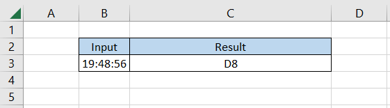
| D8 | h:mm:ss |
So let’s say there was a time value in Excel as 19:48:56 PM in cell B3, then the expected value in cell C3 using the formula =CELL("format",B3) should be D8.
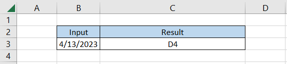
If it were a date value in mm/dd/yy format, then the expected value would be D4. The function gives the same result when we use the formula as =CELL("format",B3).
g. parentheses
When the cell is formatted with parentheses, the function returns the result as 1, or the value will equal zero.
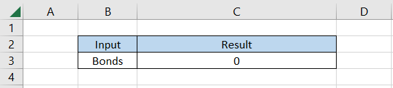
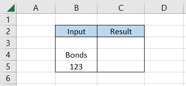
For example, suppose the value in cell B3 is ‘Bonds.’
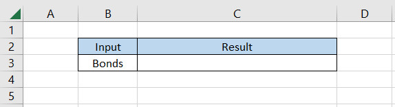
When we use the formula =CELL("parentheses",B3) in cell C3, the function returns the result as 0. This means that the cell is not formatted using parentheses.
h. prefix
When the argument ‘prefix’ is used, it checks how the text is aligned in a given cell. The function can return different symbols/characters depending on how a text value is aligned in the cell.
- Left-aligned text will be represented by a single quotation mark(‘)
- Right-aligned text will be represented by a double quotation mark(“)
- Centrally aligned text will be shown as a carat(^)
- Fill-aligned text will be backslash(\)
- An empty string for everything else
If the formula references a numeric value containing a cell, the function returns the result as an empty string regardless of the alignment type.
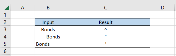
Suppose we have three values, as illustrated below, wherein cell B3 has a centrally aligned text, B4 has a right-aligned text, and B5 has a left-aligned text.
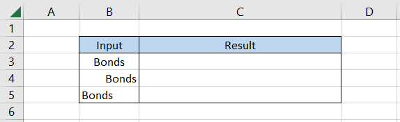
When we use the formula as =CELL("prefix",B3) in cell C3 and drag it down till cell C5, we get the result as
i. protect
The ‘protect’ argument checks if the referenced cell is locked and returns the result as 1; otherwise, as zero.
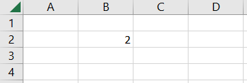
For example, suppose we have cell B2 and want to check whether it is locked. We will use the formula =CELL("protect",B2) in any cell except B2, which gives the result as 1.
This means that the cell is locked and protected in the spreadsheet. Suppose you want to check what cells are unprotected. In that case, you can use the conditional formatting tool wherein you use the formula as =CELL(“protect”,B2)=0 in the dialog box as illustrated below:
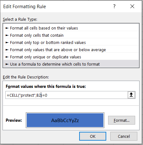
This will highlight any unprotected cells in the spreadsheet. The reference in the formula will change depending on what data you need to evaluate for unprotected cells.
j. row
As simple as it sounds, the ‘row’ argument returns the row number for any referenced cell. For example, if you refer to cell B2 using the formula =CELL("row",B2) in cell C2, the function returns the result as 2.
The argument is quite similar to ‘column,’ which returns the column number for the referenced cell.
k. type
The ‘type’ argument returns the data type in a given cell. Typically, you should expect three different data types when using the argument:
- Blank cells represented by ‘b’ (blanks)
- Text constants represented by ‘l’ (label)
- Anything else will be ‘v’ (value)
For example, suppose you have three different values in Excel, as illustrated below:
When we use the formula as =CELL("type",B3) in cell C3 and drag it down till cell C5, we get the result as
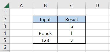
As stated above, our results match depending on the data type represented in column C.
l. width
The ‘width’ argument returns the width of the column in which the referenced cell falls. For example, if we reference the cell B2 in formula =CELL("width",B2), which is a constituent of column B, we get the result as 9.
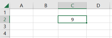
This means that the cell width of cell B2 is equal to 9, which can be confirmed by pressing the keyboard keys Alt + H + O + W, which displays the window as
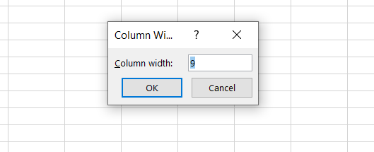
An important thing to remember is that the function rounds the column width to the nearest integer, so if the value is 9.58, the display window will show the number as 10.
Practical Examples of Cell Function
This section will see examples of using the CELL function in daily life scenarios.
a. Returning the cell address for the lookup value
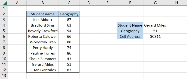
Suppose you have the data for the student’s test scores as illustrated below:
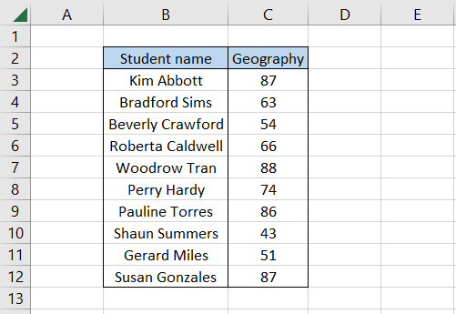
We need to find the test score for ‘Gerard Miles’ from the given data set and the corresponding cell address in which the test score is present.
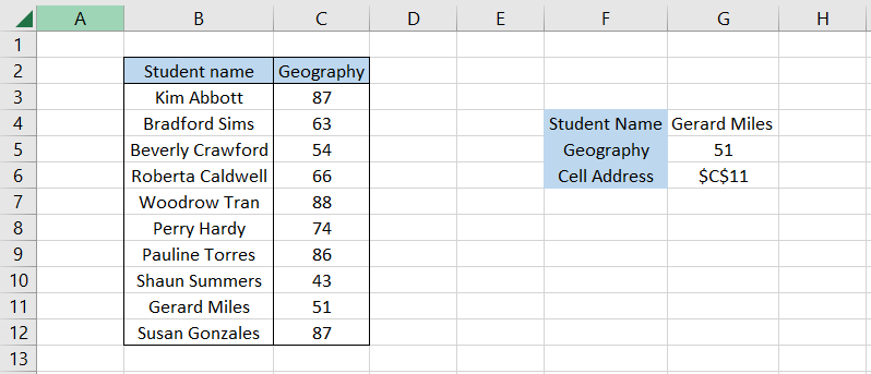
For this, we will first use the formula
=INDEX($C$3:$C$12,MATCH(G4,$B$3:$B$12,0))
in cell G5, which gives the result as 51.
However, what if there were a couple of 51’s in the data set?
This is where the CELL function plays a critical role. Just nest the INDEX MATCH formula inside the CELL function such that the formula becomes
=CELL("address",INDEX($C$3:$C$12,MATCH(G4,$B$3:$B$12,0)))
to give the result as $C$11.
Thus, you can easily find the address for any lookup value using the INDEX MATCH combination.
b. Adding hyperlinks to cell addresses returned
If we are to go one step ahead using the INDEX MATCH function, we can add a hyperlink to jump onto the cells containing the lookup value quickly.
Suppose the results that we derived were as illustrated below:
The formula further gets tweaked as =HYPERLINK("#"&CELL("address",INDEX($C$3:$C$12,MATCH(G4,$B$3:$B$12,0)))), which adds the hyperlink to lookup value as
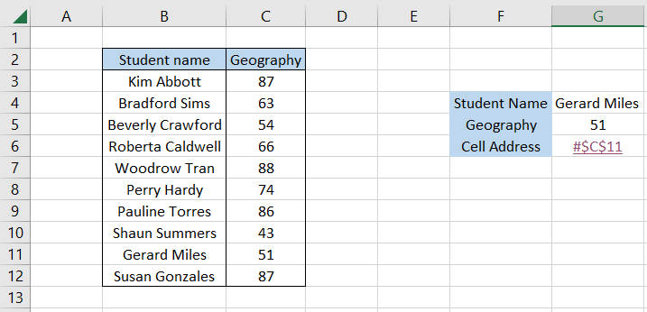
Now, if you click on the value in cell G6, it will automatically take you to the C11 cell, which has the test score for Gerard Miles as 51.

Free Resources
To continue learning and advancing your career, check out these additional helpful WSO resources:


or Want to Sign up with your social account?