CODE Function

The CODE function returns the ANSI (American National Standards Institute) code for the first character of a text string in Excel. The ANSI code is a numeric value that corresponds to the particular character in the ANSI character set.

Before the UNICODE function, the ANSI character set was a standard used in Windows OS through version 95 and Windows NT.

ANSI was initially a set of 217 characters, also called Windows-1252, eventually adding the euro currency symbol, bringing the current total to 218.

Since Excel uses these character sets in its function, each of these characters corresponds to a specific number. As a financial analyst, you can use the CODE function to take a particular action on a recurring character from this character set.

Since the function only needs the first character while ignoring the rest of the text string, it rules out the possibility of additional ANSI values or incorrect values.

CODE function: What is it?

It is categorized as a text function that returns a numerical value corresponding to one of the characters in the ANSI character set adopted by Excel.

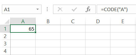
For example, when you input the letter 'A' inside the function, you will get 65. This means that the numerical code for capitalized 'A' is 65.

Similarly, if you input a lowercase 'a' as an argument in the function, you will get 97.

This little exercise can reveal a significant revelation: all the unique characters will have special numerical codes. This includes the capitalized alphabet and its lowercase counterpart.

CODE is a built-in function and can also be accessed from the Formulas tab as a worksheet function.

To use the function from the formulas tab, please follow the instructions below:

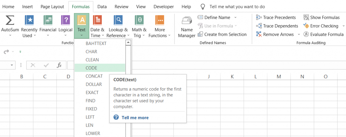
• Select the cell in which you want to use the function, click on the Formulas tab, and then on text in the function library.
• In the drop-down, select the CODE function. This will open up the window as illustrated below:
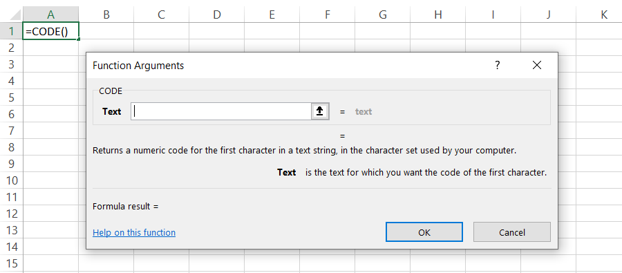
• We will input the text as 'A' and click on OK. This will give us the result in cell A1 as:
• Try following the same method but input the text as 'Amazon Inc.' this time. We will get the same result:
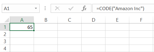
• From this example, we learn the function will only capture the first character of the text string and return its corresponding numerical value.
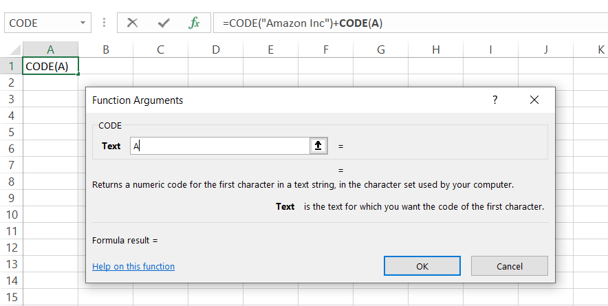
• It is important to remember to remove the existing CODE function in the cell before using it again if the argument is hard coded. As you can see, if we select the same cell for a process, the result gets added up, which can give a misleading numerical value. 
  Here, instead of the result being 65 for capitalized 'A,' we get the numerical code as 130, which is the sum of two capitalized 'A's.

If you don't prefer using CODE as a function, you can also use it as a formula in the cell of the worksheet.

The syntax for the CODE function:

=CODE(text)

where,

text = (required) text string for which we need to return the numeric code

Note: Naturally, you will have text strings with more than one character. The function only captures the first character and returns the corresponding ANSI character code while ignoring the rest of the text string.

Examples

As we now understand the syntax for the function, we will look at a couple of examples of how you can use the process in Excel.

Example #1

To use the function as a worksheet formula, we begin with the equal sign and type in the function name. Then, inside the parentheses, you can either hardcode a value or make the formula dynamic by inserting a cell reference.

To understand how the formula works, we will see what code the function returns for various alphabetical characters. For example, the data in Excel looks as illustrated below:

To find the code for each character, we will use the formula

=CODE(B3)

Which will give us the result:

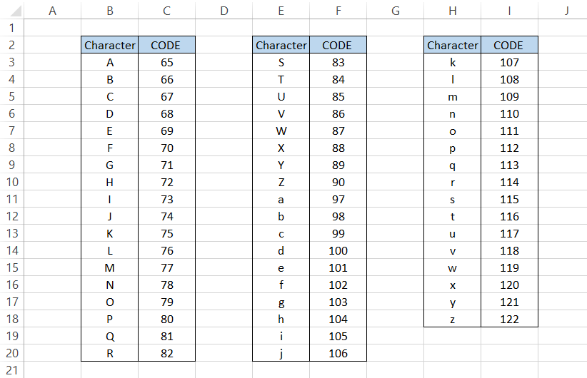
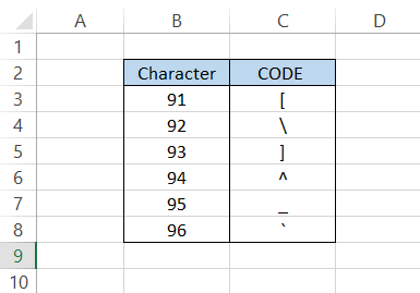
We can draw information from the result that the numerical codes for the capitalized alphabet are between 65 and 90, while the lowercase letters go from 97 to 122.

What are the numbers 91-96? Why did the numbers directly jump from 90 to 97?

Well, that's because another set of characters has those numerical values. So the collection of characters is:

Example #2

If the function returns a numerical code due to different characters in Excel, what would happen if we input numbers?

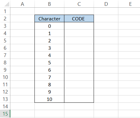
Let's say we have numbers from 0 to 10 in a spreadsheet, as illustrated below:

By using the formula

=CODE(B3)

In cell C3 and dragging it down to cell C13, we will get the result:

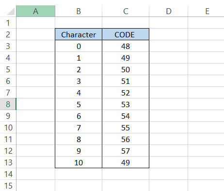
You would still get their corresponding numerical code when you input numbers inside the formula. For example, in the ANSI set of characters, the value of zero (0) equals 48. Therefore, one (1) has been assigned 49, and so on.

As you might have already noticed, once the double-digit numbers start, we get the result corresponding to the number's first digit. This is because the function ignores all the numbers to the right, giving us a result of 49 in cell C13.

Example #3

What would happen if you had a text string enclosed inside quotation marks?

So far, we have only seen the cells with text without quotation marks.

Suppose you have the text in cell B2 as "Elon Musk is the CEO of Tesla Motors."

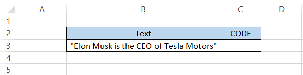
Anyone who has skipped several sections of this article would think, "Yea, 'E' is the first character of the text string, so that the numerical value would correspond to the letter E."

Well

Before the first letter, we have another character in quotation marks ("").

So, by using the formula

=CODE(B3)

the expected result in cell C3 would be 34, the ANSI code for a quotation mark, instead of 69 for the letter E.

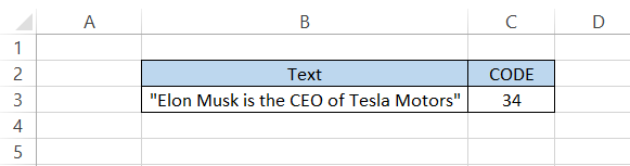
Even if you hardcode the text inside the formula, i.e., make the formula =CODE("Elon Musk is the CEO of Tesla Motors"), you will get the same result.

CHAR function - an inverse of CODE

We love working with the CODE function and what it can achieve, even though it has its limitations. So it was only logical that our curiosity got the better of us.

You can use the CODE function to return the numerical value for different characters in Excel. But half the time, we don't even know where the various symbols/feelings on the keyboard are.

This made us think about how we could return the character based on its numerical counterpart. But it had its downside. You must first know the numerical code for the surface you intend to return.

This can be achieved with the help of the fantastic CHAR function. The function returns a character when inputting a character code inside the part. CHAR is a short form for the 'character' function.

The syntax for the function is:

=CHAR(number)

where,

number = (required) number for which a corresponding character would be returned

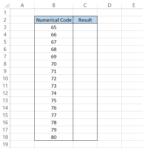
Suppose that you have numbers in Excel from 65 to 80, as illustrated below:

By using the formula

=CHAR(B3)

The corresponding numbers will give us the characters in Excel:

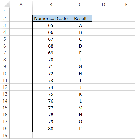
Those are the numbers from where the alphabet begins, but, again, the function works when you know the different numbers for the corresponding character.

If you need help with what numbers return which characters, you can use the official documentation offered by Microsoft for the numbers and their character counterparts.

Practical Example #1

Suppose that you work at a bank, and your bank agrees to provide loans to 25 borrowers:

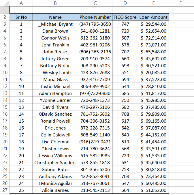
The raw data file has some inconsistencies, and you need to remove those inconsistencies before you can upload the raw data into the database.

Suppose that the inconsistencies in the phone numbers are the round brackets you can see at the beginning of the numbers.

To highlight all the phone numbers with such inconsistencies, we can first use the LEFT function to get the character.

The LEFT function will extract the character, which can be assessed to determine the phone number's inconsistencies.

The formula will be

=CODE(C3)

giving the result as 40. Luckily we had only one character that wasn't a number, so the numerical value for the parenthesis is equal to 40.

If you don't need to assess the beginning characters, you can directly skip the step and find their numerical value.

Next, we nest the result inside the IF function such that if a similar character occurs in the succeeding phone numbers, the TRUE result will caution us about the existence of such inconsistencies.

The formula to check the cells with irregular phone number formats is =IF(CODE(C3)=40, "Formatting is wrong,""), which will give you the result as illustrated below:

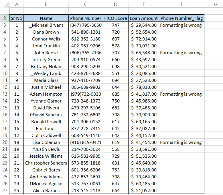
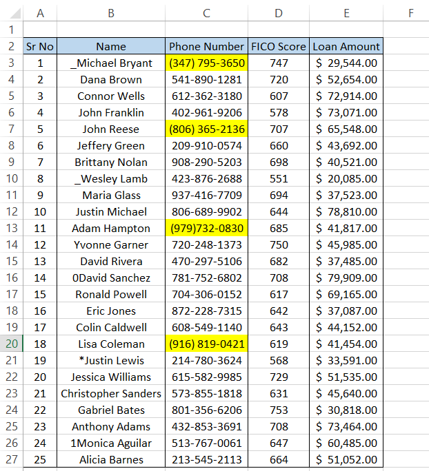
As you can see, in four instances, we had the parenthesis character before our phone numbers, a phone number format that our database cannot accept.

All those phone numbers can be corrected, and then the data can pass on to the database.

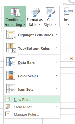
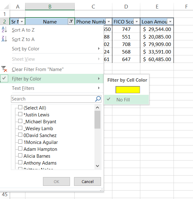
Another alternative that you can use is the conditional formatting tool. For example, select the range C3:C27 and click on the dependent formatting tool from the Home tab.

Select 'New Rule' from the drop box.

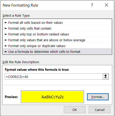
This will open up the dialog box for the 'New Formatting Rule.' We will use the formula as =CODE(C3)=40, use a fill color to highlight the cells, and click on OK.

This should give you the result as illustrated below:

Similarly, we know that the numerical values for capital letters go from 65 to 90, and for lowercase letters, it is from 97 to 122.

To find any irregularities at the beginning of the 'Name' column, the formula that will be used in the Conditional Formatting Tool will be

=OR(AND(CODE(B3)>=65, CODE(B3)<=90), AND(CODE(B3)>=97, CODE(B3)<=122))

which will highlight only the cells that have proper formatting without non-letter characters at the beginning.

Based on the color code, you can further sort the data based on 'No Fill.'

This will finally give you the result as illustrated below:

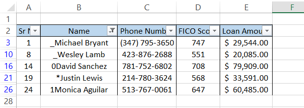
You can now make the changes and follow the same steps again to check for any irregularities in the data.

Though the method looks very tempting to use, remember that the function will not consider any irregularities in the middle or at the end of the data.

The function can work wonders if you are OK with only catching flaws at the beginning of the text string (a limited application).

Important things to remember:

• The function accepts only one argument, which takes in the text string's first character, returning a corresponding numerical code.
• You will get a #VALUE! Error when the text argument is left empty
• The CHARS function performs the inverse of the task the CODE function performs. It will return the character based on the numerical value you input into the function.
• The output for the function will be different in different operating systems.

If a text string enclosed in quotation marks (or any other character) is passed through the function, we will get the numerical code for the quotation marks rather than the first character of the text string.

Researched and authored by Akash Bagul | LinkedIn

Reviewed and edited by James Fazeli-Sinaki | LinkedIn

Free Resources

To continue learning and advancing your career, check out these additional helpful WSO resources:

• HOUR Function
• HYPERLINK Function
• PEARSON Function
• PI Function
• SEARCH Function