CHAR Function

What is the CHAR Function?

The CHAR function in Excel returns the corresponding character based on the ANSI (American National Standards Institute) code you input. The ANSI code is a numeric value that corresponds to a particular character in the ANSI character set.

ANSI was initially a set of 217 characters, also called the Windows-1252, eventually adding the euro currency symbol taking the count to 218.

Since all these characters are used in Excel, each one is assigned a unique number as an identifier. If you know what number corresponds to a particular character, then you can use the function to input that character in Excel easily.

You can also make logical conditions on the numbers corresponding to those characters. For example, if those characters are found in a text string, then using the numbers, you can return one result(when evaluation is TRUE) and another(when evaluation is FALSE).

In this section, we will see the CHAR function, its syntax, and a couple of examples to understand it better.

Understanding CHAR function

CHAR is categorized as a Text function that returns the corresponding character from the ANSI character set based on the number you input in Excel.

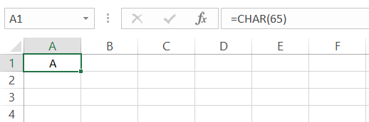
For example, when you input the number 65 inside the function, you will get the result as the alphabet 'A.'

Similarly, if you input the number 97, you will get the result as a lowercase 'a.'

You would get all the unique characters assigned to those corresponding numbers based on the number you input in the function.

Since there are no two same numbers, the characters do not repeat for any of them. This is why we have different numbers for the upper case 'A' and lower chance 'a.'

The CHAR is a built-in function and can also be accessed from the Formulas tab.

To use the function from the formulas tab, please follow the steps below:

1. First, select the cell in which you want the result. 
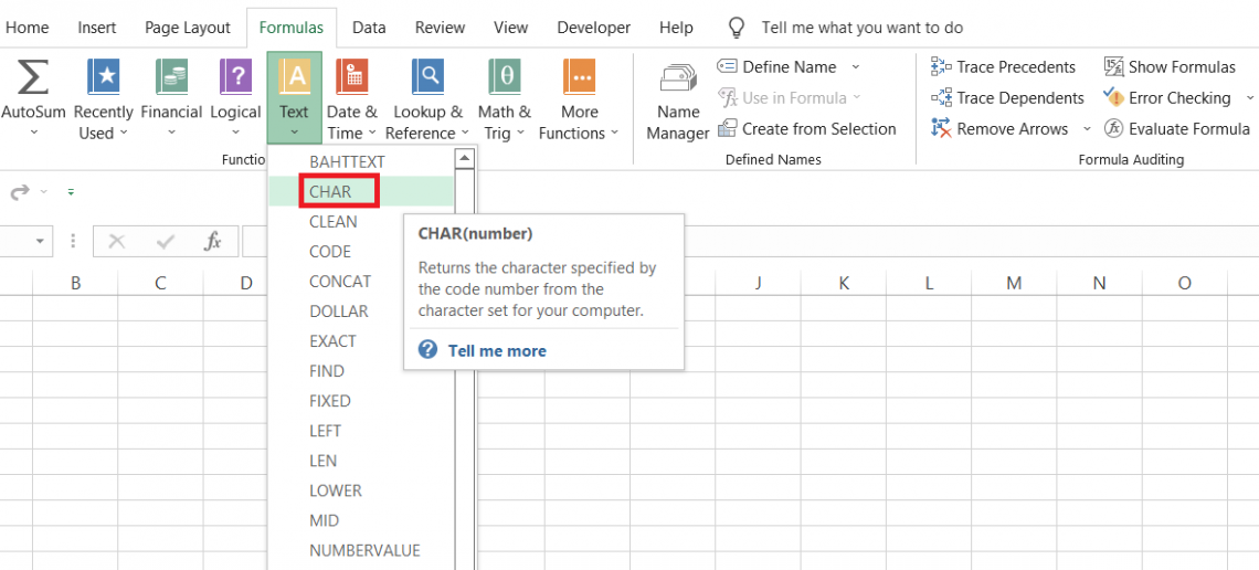
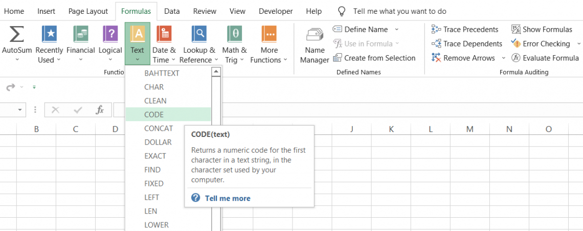
2. Click on the Formulas tab > Text > select the CHAR function from the drop-down menu. This will open up the dialog box, as illustrated below:
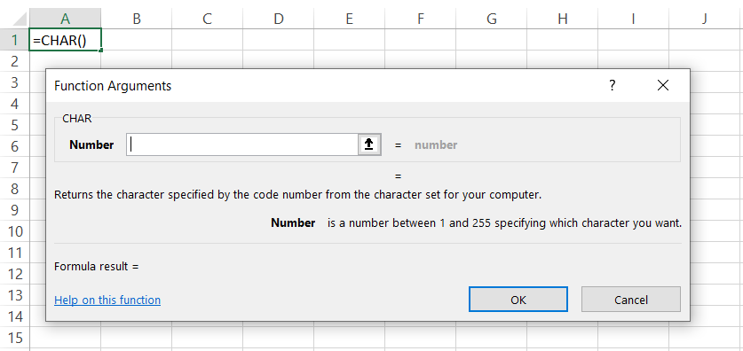
3. As stated in the description, the number can be anything between 1 and 255 that will return the specific character for you. For example, suppose we input the number 65.
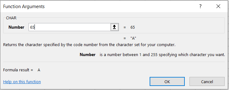
4. When we click on Ok, we get the result as 'A' in the selected cell.
5. Let's see the result when the input is more significant than 255. For example, suppose the number we input is 278. Then, when you click on OK, you will get the #VALUE! Error.
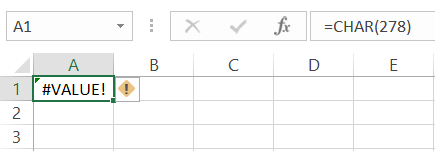
6. From this, we can interpret that we can only use numbers from 1 to 255, and anything above or below them will return a #VALUE! Error.

If you don't prefer to use the CHAR function from the library, you can also use it as a worksheet formula.

The syntax for the function is:

=CHAR(number)

where,

• number = (required)any number between 1 and 255 that corresponds to the specific character 

Examples of the CHAR function

We saw the syntax for the function and how to use it from the function's library. This section will show examples of how you can use the formula as a worksheet.

Example #1

To use the function as a worksheet formula, we begin with an equal sign, type in the function name, and input the argument inside the parentheses. The idea can either be hardcoded or a cell reference containing the input value.

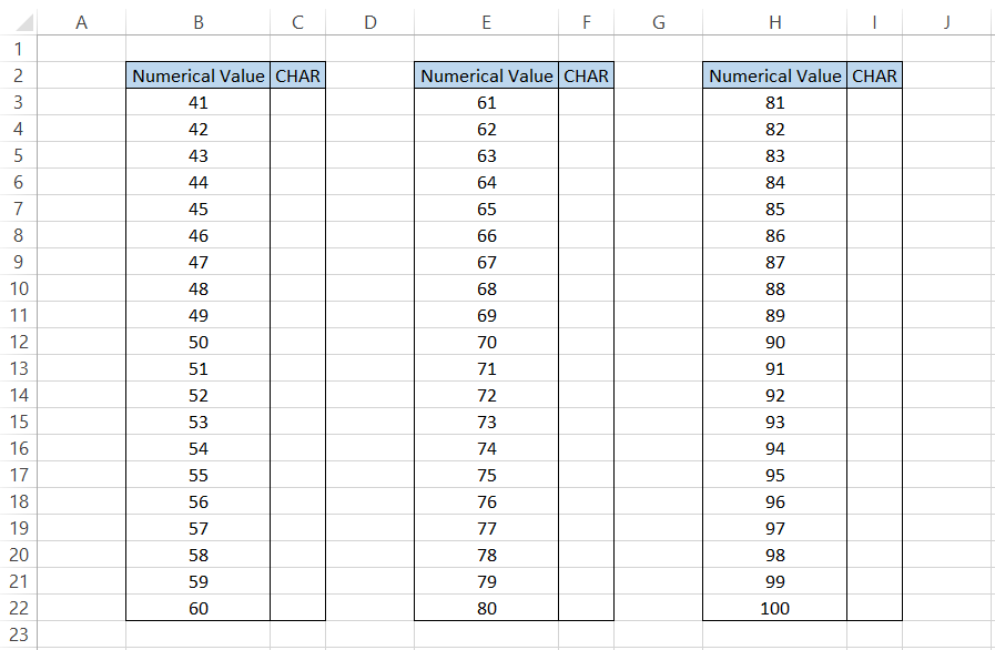
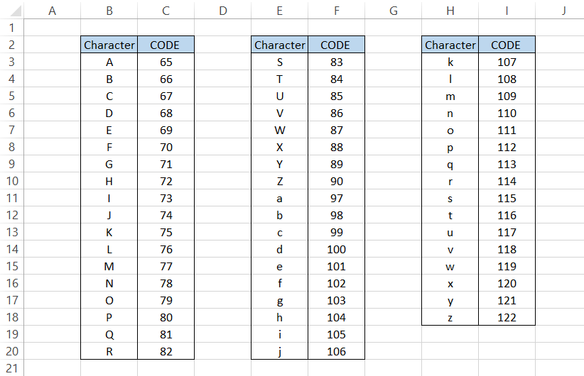
To understand how the function works, we will see what character the function returns for the numbers between 41 and 100. The data in Excel looks, as illustrated below:

To find the character for each numerical value, we will use the formula =CHAR(B3) in cell C3 and copy it into all the respective columns. This will give us the result:

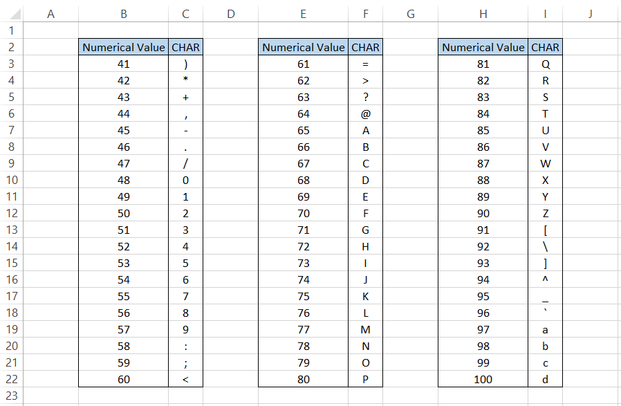
We notice that the capitalized alphabets begin from the number 65 and end at 90, while the lowercase alphabets start from the number 97.

The numbers between those two, i.e., from 91 to 96, are assigned to another set of characters.

You might also notice that sometimes the function cannot display the character even after using the process.

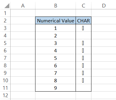
These are some of the characters that are unavailable in the Excel library. Also, you can check out the ASCII Table to understand those values and determine if getting characters corresponding to those numbers was possible!

Example #2

What would happen if you text string as an argument for the function?

Suppose you have the data as:

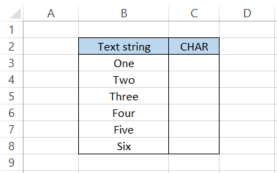
If you use the formula =CHAR(B3) in cell C3 and drag it down to cell C8, you will get the #VALUE! Error.

The interpretation from this example is that the function will only accept numerical values between 1 to 255, while all the numbers beyond that and the text strings will return a #VALUE! Error.

Example #3

What about the result of the characters?

Well, it only makes sense if we know all the characters that correspond to 255 characters.

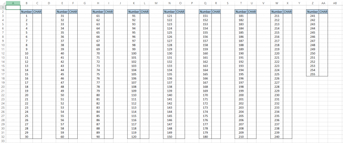
As usual, we will use the formula =CHAR(B3) in cell C3 and copy it to all the cells to get the result, as illustrated below:

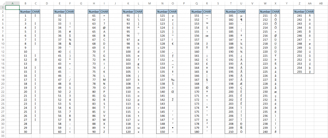
Here, you can get a clear view of the different characters that are missing in the set and characters that Excel cannot display(represented by a vertical rectangular prism).

If you cannot find any character on the keyboard, you can easily use the function to get that character after the text string.

For example, let's assume you cannot find the question mark on the keyboard. The numerical value that corresponds to the character is 63.

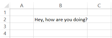
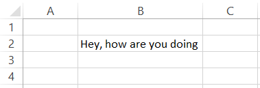
If the text string is 'Hey, how are you doing,' then all you need to do is use the formula = "Hey, how are you doing "&CHAR(63), and you will get the result:

This way, you can include any character with the text string by concatenating the function along with the text string.

CODE function - Inverse of CHAR

All the 255 numbers are helpful as long as we are aware of what the corresponding characters are.

But sometimes, the characters are already present in Excel, and we might need to take some action based on the presence of those characters.

What can we do then?

This can be achieved with the help of the CODE function. The function is categorized as a Text function that returns a numerical value corresponding to the character from the ANSI character set.

The syntax for the function is:

=CODE(text)

where,

• text = (required) text string for which we need to return the numeric code

To understand how the function works, we will see what code the function returns for various alphabetical characters. The data looks as illustrated below:

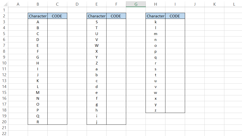
To find the numerical code for each alphabet, we will use the formula =CODE(B3), which will give us the result:

We can interpret that the numerical code for the capitalized letters is from 65 to 90, while for the lowercase letters, it is between 97 and 112.

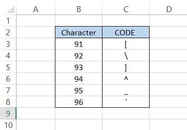
You might be wondering what about the numbers between 91 to 96?

Well, that's because another set of characters is assigned to those numbers, as illustrated below:

CHAR Function - Practical Example #1

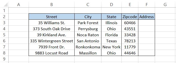
Suppose you have some of the addresses in Excel. Then, you need to combine the lesson so that each speech component is represented on a different line.

Now, if you directly concatenate the components and then keep pressing the Alt + Enter for a line break, it might take a lot of time.

However, the other alternative is to add the line break using the CHAR function.

The data looks as illustrated below:

Here, we will use the formula =B3&CHAR(10)&C3&CHAR(10)&" "&D3&" "&E3 in cell F3 and drag it down to cell F8, which gives us the result:

What? Shouldn't that have worked to give us the line breaks?

Yeah, right. One more thing we need to do before the formula works is wrap the text. We will select the range F3:F8 and use the keyboard shortcut of Alt + H + W, which finally gives the result:

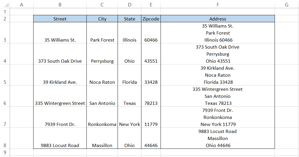
It may not look much, but the line break character with a numerical value equal to 10 can be instrumental when you are looking to represent the data in different lines!

CHAR Function - Practical Example #2

In this example, we will try to combine the CHAR and the CODE functions, which are inverse.

Suppose you download an Excel file from the internet that has the text strings, as illustrated below:

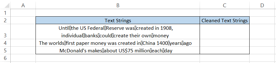
As you might have noticed, we have additional characters in an unrecognizable format inside the text strings.

To remove them, we will use the formula =SUBSTITUTE(B3,CHAR(CODE(""))," ") in cell C3 and drag it down to cell C5, we get the result:

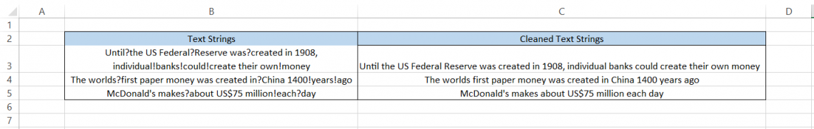
All the additional characters in the text string get replaced by the space character.

How does the formula work exactly?

• We know that the CODE function requires the input of a character, whereas the CHAR function requires the information of a number to get the feeling.
• Based on the same logic, we first use the CODE function and copy the unknown character into the CODE function, which ultimately gets us the numerical counterpart.
• Now, the CHAR function will give us the same character, which gets substituted by the space character in our text string to provide us with the cleaned text string.

Even though the CHAR and code functions have much less practical usage, you never know when you might need to use the process!

Researched and authored by Akash Bagul | LinkedIn

Reviewed and edited by Parul Gupta | LinkedIn

Free Resources

To continue learning and advancing your career, check out these additional helpful WSO resources:

• HOUR Function
• HYPERLINK Function
• PEARSON Function
• PI Function
• SEARCH Function