EXACT Function

What is the EXACT Function?

The EXACT is a case-sensitive function that compares two supplied test strings and returns the result as TRUE if they are an exact match and FALSE if they do not match.

There are instances when you need to check whether a particular value has a precise match in the thousands of rows of data.

Some would argue that aren't 'excel' and 'Excel' the same. They are, but they differ in one particular part: the beginning letter. The word 'excel' has a lower cased letter while 'Excel' has a capitalized letter.

And even though they have the same number of letters, if you want to evaluate the word 'excel' and only find a precise match beginning with a lowercase letter, you need to use the function.

The function is used because without its help; Excel would identify both of them as equal, i.e., 'Excel' = 'excel.'

Let's not get too technical already. First, we will see the function, its syntax, and how to use it, along with a couple of examples.

Understanding the EXACT function

The function is categorized as a Text function that will help you make case-sensitive comparisons between different supplied text strings and return the result as a boolean value.

For example, when you use the function for text strings 'Apple Inc' and 'apple inc,' the process evaluates the comparison as FALSE since they both have capitalized and lowercase beginning letters, respectively.

However, if the two strings were 'Apple Inc' and 'Apple Inc,' the function would return the result for the comparison as TRUE.

In the absence of the function, Excel would have returned the boolean value as TRUE in both cases since, by default, it doesn't make case-sensitive comparisons.

The use of function can be highly beneficial where you have similar values that might differ based on the capitalization of different letters in those text strings.

EXACT function Formula

The syntax for the function is:

=EXACT(text1, text2)

where,

• text1 - (required) reference to the first text string
• text2 - (required) reference to the second text string

How to use the EXACT Function in Excel?

You can use the function in two ways - either from the function's library or as a worksheet formula.

Most Analyst/ Investment bankers prefer using the formula as a worksheet function since they offer more flexibility in making different operations on the cell values.

1. From the function's library

Even Naruto started as a genin before becoming a Hokage for the hidden leaf village. So if you want to become an Excel wizard, we advise you to at least start understanding the arguments for different functions from the library.

To use the function from the library, please follow the steps below:

1. First, select the cell where you intend to get the result for the process.
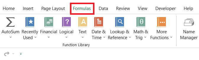
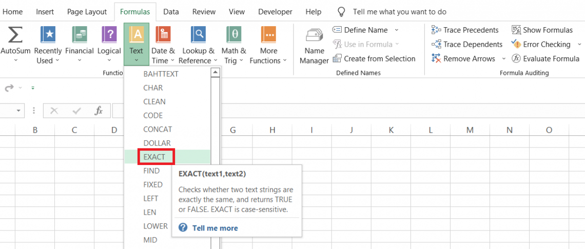
2. Next, click Formulas > Text > select the EXACT function from the drop-down menu.
3. This will open up the dialog box, as illustrated below:
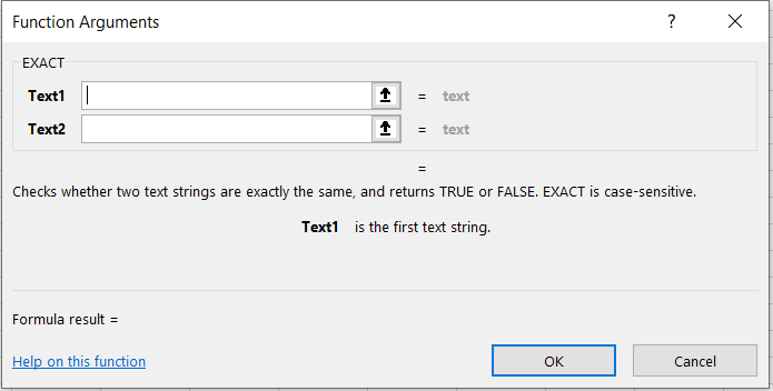
4. Here, you input the text strings either as a hardcoded value or as the cell references from the spreadsheet.
   We will input the two text values as 'Stock' and 'Stock,' as illustrated below: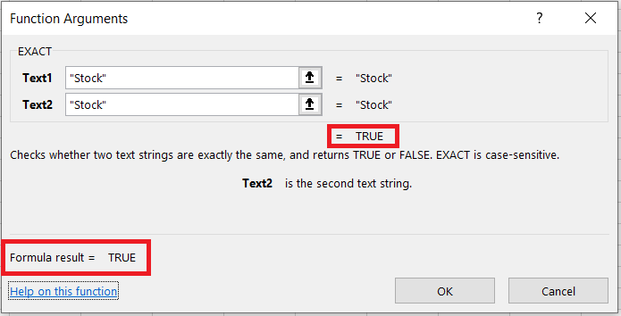
5. When we input all the arguments in the dialog box, we already get the result preview in the same window.
6. When you click on Ok, you will get the same result in the selected, i.e., the boolean value as TRUE.

2. As a worksheet formula

The easier of the two methods and probably the more preferred if you have intermediate skills in Excel.

All you need to do is select the cell, begin with an equal sign, type in the function name and finally input the argument inside the parentheses.

Suppose that you have the data as illustrated below:

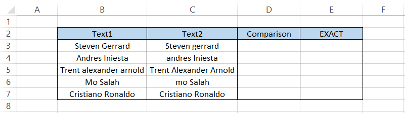
Then, in column C, we will make a standard comparison, i.e., =Text1=Text2, to check whether both values are equal. 

The formula that we will use in cell D3 is =B3=C3 and drag it down to cell D7, which gives us the result:

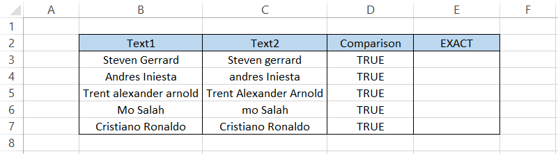
As you can see, even though the beginning letters for the first and last name are not capitalized, the general comparison still gets us the result as TRUE since the compared values have the same number of letters.

On the other hand, when you use the formula =EXACT(B3, C3) in cell E3 and drag it down to cell E7, you would get a contrasting result:

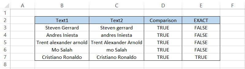
Only in one instance do we get the result as TRUE for 'Cristiano Ronaldo' where all the upper and lower case letters match each other in compared values and the total number of letters in each text string.

EXACT Function Example

The function is hugely resourceful when used in or combined with some other process.

The function works well with other functions such as IF statements, SUMPRODUCT, OR, AND, MID functions, etc.

These functions do not belong to a single category; some are logical functions, and some are statistical functions, including text functions. This portrays the versatility of the EXACT position and the vital role it can play in data analysis if used appropriately. 

The functions and data validation tool can be used via formulas to get the 'exact' results. 

This section will provide examples to help us understand how we can best use the function.

Example 1: Just the EXACT function

You don't always need to work on complicated tasks to prove the function's usefulness.

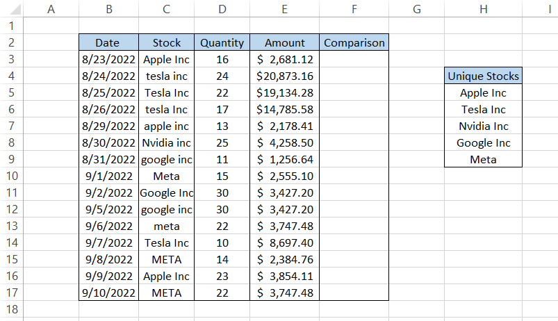
Suppose you work at a Mutual fund and need to store the data for all the transactions. For example, the data for all the trades taken for the last fifteen days are as follows:

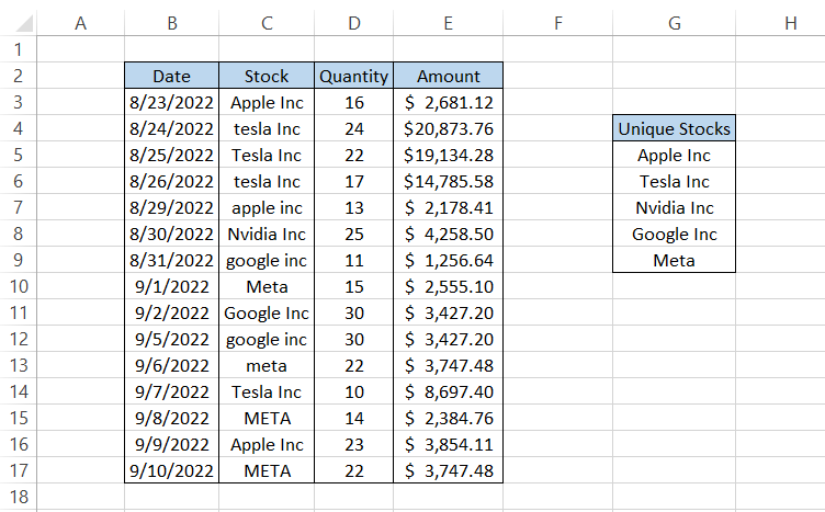
All the unique stock names are stored in column G, i.e., five individual stocks based on all the trades you took.

As you might have already noticed, much of our data is inconsistent in column C. The reason to check these inconsistencies is the database only accepts text strings that are already calibrated in the system, which are in column G

So what can you do then?

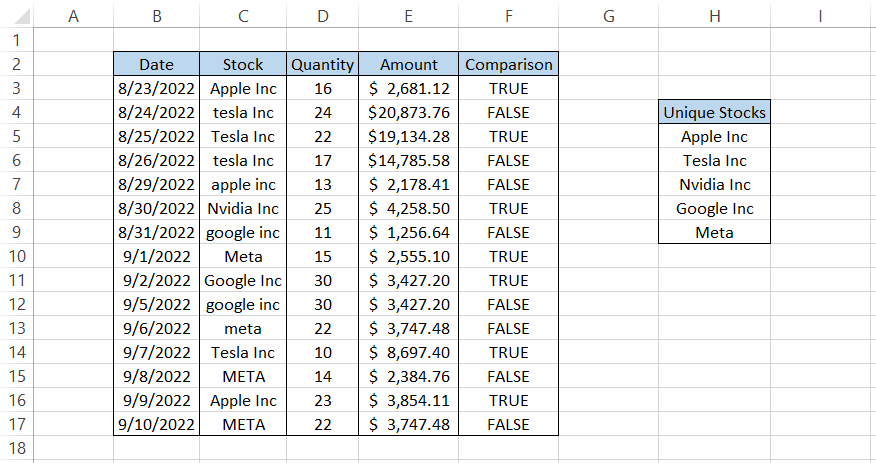
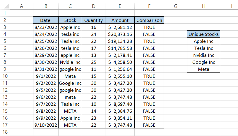
It's best to check whether all the text strings are consistent in the initial steps. Here, we will create an additional column and use the function to compare the two text strings in columns C and F, respectively.

We will use the formula =EXACT(C3, VLOOKUP(C3,$H$4:$H$9,1, FALSE)), which compares the text string in column C to that in column H.

If a precise match is found, then the formula returns as TRUE. If not, the procedure returns as FALSE.

Since some of those formulas evaluate FALSE, we can immediately substitute those with the values in column H. Once done, you will get all the procedure results in the 'Comparison' column as TRUE.

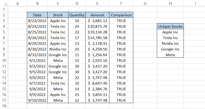
The text strings in their acceptable form can then be uploaded onto the database you have maintained for all the trades in the bank.

Example 2: Along with the SUMPRODUCT function

Another function that works great in combination with EXACT is the SUMPRODUCT function.

The SUMPRODUCT function returns the sum of the products by multiplying two or more ranges or arrays together.

Suppose the bank you work at made a series of buy transactions for tesla stock.

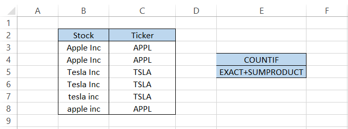
If you use the traditional non-case-sensitive COUNTIF function to find the total 'Tesla Inc' stocks using the formula =COUNTIF(B3:B8, "Tesla Inc"), you will get the count equal to 3.

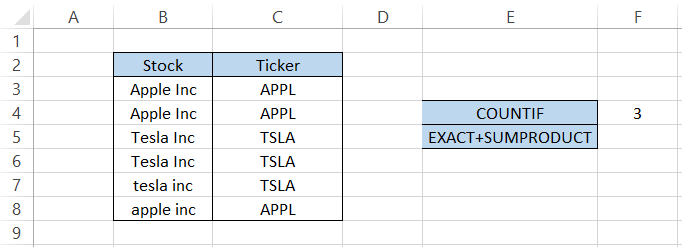
Notice that cell B7's text string starts with the lowercase 't' while the other two values have an uppercase 'T.' However, even after this anomaly, the function captured all the text strings with the same alphabet as 'Tesla inc.'

However, if you use the formula =SUMPRODUCT(--EXACT(B3:B8, "Tesla Inc")), we get a contradictory result, which is equal to 2.

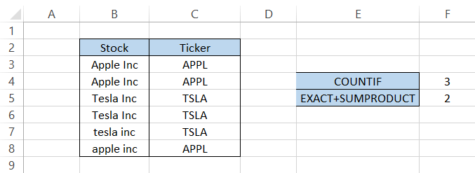
The formula ignores the text string with the lower case 't,' i.e., tesla inc, and only counts the other two values in the range.

This way, you can use SUMPRODUCT and EXACT functions to make case-sensitive counts in Excel.

Example 3: With the IF function

Did you think we were going to forget the IF function?

Any function that returns the result as a boolean value, i.e., TRUE or FALSE, can be combined with the IF statements.

The IF statements will return a user-customized result when the boolean value equals TRUE and a different customized result when the value is FALSE.

Let's return to one of our previous examples where we want to store the data in our database.

Using the formula =EXACT(C3, VLOOKUP(C3,$H$4:$H$9,1, FALSE)), we get the result as a boolean value in column F.

What we would do is nest the entire formula inside the IF statement such that the whole formula becomes =IF(EXACT(C3, VLOOKUP(C3,$H$4:$H$9,1, FALSE)), "Text strings do not match"," "), which gives us the result:

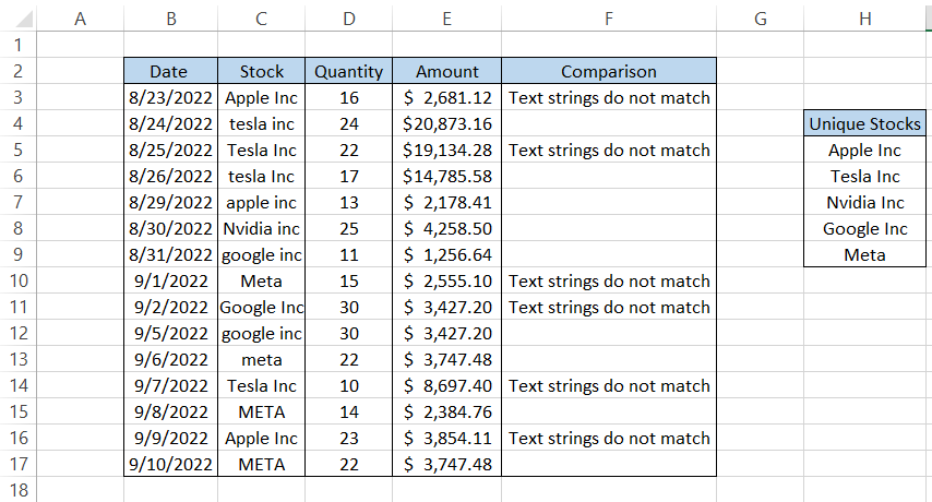
Whenever the formula evaluates to TRUE, we get a custom text string 'Text strings do not match as our result, whereas when the formula evaluates to FALSE, we get an empty string.

Example 4: With the Data validation tool

If your organization stores a lot of internal data in Excel, you need proper formatting in those files before they are uploaded to data management software such as SQL.

In such a case, you can use the data validation tool to accept text strings beginning in the upper case.

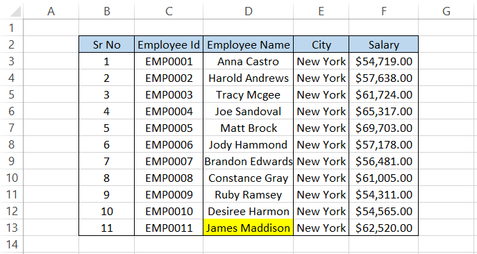
Suppose you have the data, as illustrated below:

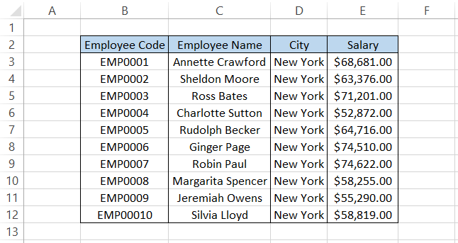
If a new employee joins the company, we only wish to enter the data in the 'proper' case.

To do so, select the entire column starting from cell C3(exclude the first two rows, not that it matters).

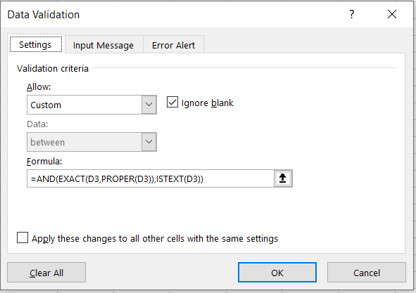
Click on the data> Data Validation and set Validation criteria to Custom, which should show the Formula dialog box.

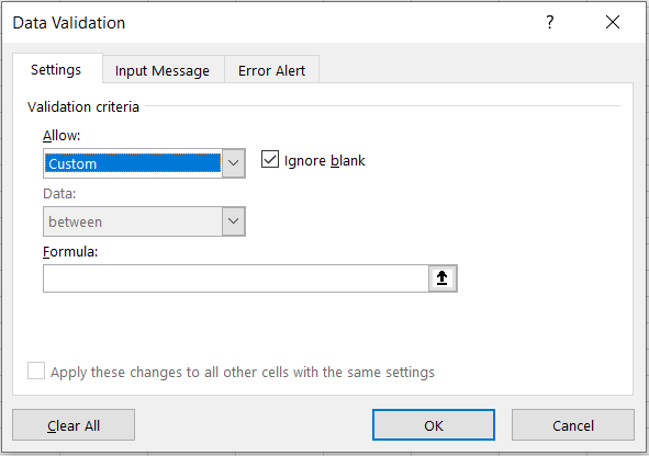
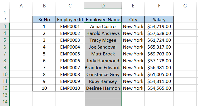
Here, we will input the formula as =AND(EXACT(D3, PROPER(D3)),ISTEXT(D3)) and click on Ok.

Now, enter the employee details usually in Excel, and you will find that if the 'Employee Name' is not in the proper case, then we get an Excel error, as illustrated below:

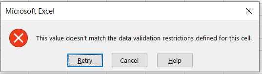
For example, if the name is 'James Maddison', the cell won't accept the name as 'James Maddison,' 'James Maddison, ' or even as 'JAMES MADDISON.'

If you have similar data columns in Excel, for example, 'City,' you can follow the same procedure to add the data validation restrictions to those columns.

The only question to be answered is - how the formula works.

• The EXACT(D3,PROPER(D3) part evaluates whether the text string you input is in the proper case. If it is, this part of the formula considers TRUE or else FALSE.
• The ISTEXT(D3) returns TRUE when you input text and FALSE when it is not.
• The AND function combines TRUE results and only accepts the value we input in column D.

Example 5: Find the match with OR

Finding a precise match from the list using the VLOOKUP in the formula is a good option. But what is another more accessible alternative that you can use?

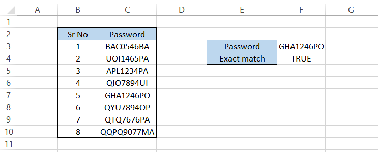
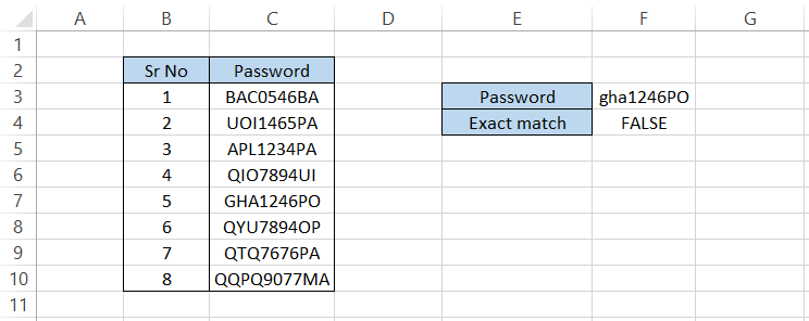
Suppose that you have some of the passwords in Excel as below:

The value in cell F3 represents the password we are looking for if it exists in our Excel data.

To get the match, we will use the formula =OR(EXACT($C$3:$C$10,F3)) in cell F4, which will give us the boolean value as TRUE or FALSE.

An essential thing to remember is that since this is an array-based formula, you need to press Ctrl + Shift + Enter to get the result.

Once you press those magic keys, you will get the result as illustrated below:

However, on closer inspection, we find that we have the same password in cell C7. So let's manipulate the password a bit and check if we get the same result.

When we input the password as 'gha1246PO', even though it is present in cell C7, we still get the result as FALSE since the beginning three letters are in lowercase and do not allow for a match.

This way, you can use the combination of OR and EXACT functions to find a match of a value from the list.

Example 6: Finding the 'non-identical' character

Finding an exact match is one thing, but there might be instances when you might need to find the character that is non-identical in the data set, which ultimately returns the result as FALSE.

In such cases, we use the combination of MID and EXACT functions.

Suppose we have the two text strings, as illustrated below:

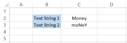
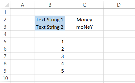
Both strings have 5 characters, so we will create a column numbered from 1 to 5.

Next, we will use the formula =EXACT(MID($C$2,B5,1),MID($C$3,B5,1)) in cell C5 and drag it down till cell C9, which will give us the result:

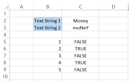
All the cells with a boolean value equal to FALSE interpret that those letters do not have a match.

How does the function work?

• We use two mid-functions that extract each letter from our word. For example, MID($C$2,B5,1) extracts the first letter from cell C2, i.e., ‘M’ and MID($C$3,B5,1) extracts the letter ‘m’ from cell C3.
• The EXACT function then compares those letters such as =EXACT('M', 'm') and evaluates to TRUE if they match and FALSE if not.
• The rest of the letters are extracted similarly to make the comparison. 

Researched and Authored by Akash Bagul | Linkedin

Reviewed and edited by Parul Gupta | LinkedIn