YEAR Function

What is the YEAR Function?

The YEAR function returns the year component from the given date in Excel. Since the dates start from 1st Jan 1900 in Excel, the year can range from anywhere between 1900 to the present or the future year, depending on the date supplied as the argument.

When you are working on extensive data and need to group the dates based on year, the function works wonders by initially extracting the year component for the user.

Once the 'criteria' are extracted, you can use either the pivot tables or sort the data in ascending or descending order to visualize the data as per your need.

While preparing financial models, one of the essential components for forecasting is the year. Once we input the fiscal year-end date in the economic model, we can easily extract the year component and further input our projection years using the EOMONTH function.

In this article, we will see the syntax for the function, how to use the process and a couple of examples.

Understanding YEAR function

The YEAR is categorized as a Date and Time function that returns the year value from the given date in Excel.

When you reference or hardcode a date inside the function, say 5-Aug-2022, the result you should expect using the process is equal to 2022.

Similarly, if you enclose the date 8/5/1901 inside the function, you would get the result as 1901.

The function extracts the year component from the date and ignores the day and month components from the date.

We have a task for you - Try to extract the year component for the dates before 1st January 1900.

Let's say the date was one from the mid-1600s when the 'tulipmania' occurred. You input the date as 8-March 1638 and then nest it inside the function as an argument. What result do you get?

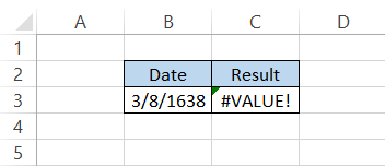
We get the #VALUE! Error as our result. As we previously discussed, the dates in Excel begin from 1st Jan 1900, and therefore any dates before that time would result in the #VALUE! Error. 

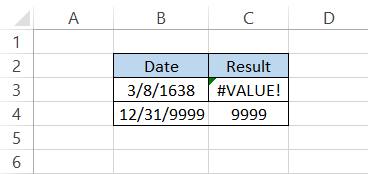
This implies that 1st Jan 1900 is our lower limit when we input dates in Excel. What do you believe is the current upper limit for the dates in Excel?

Let's say you input the date 12/31/9999 in Excel as the argument inside the function, giving you the result as 9999.

So is 9999 the upper limit for the year in Excel? Not sure yet! Let's add one year to the date of 12/31/10000. This time we get the #VALUE! The error implies that the date falls outside the range acceptable to Excel.

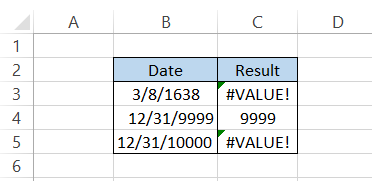
Thus, Excel can only accept date values between 1st Jan 1900 to 31st December 9999, which can be easily identified using the YEAR function.

The only question remains: What is the function's syntax?

The syntax for the YEAR function

The syntax for the function is:

=YEAR(serial_number)

where,

• serial_number - (required) a serial number, a cell containing a date, or a formula that returns the date that will be used to extract the year. 

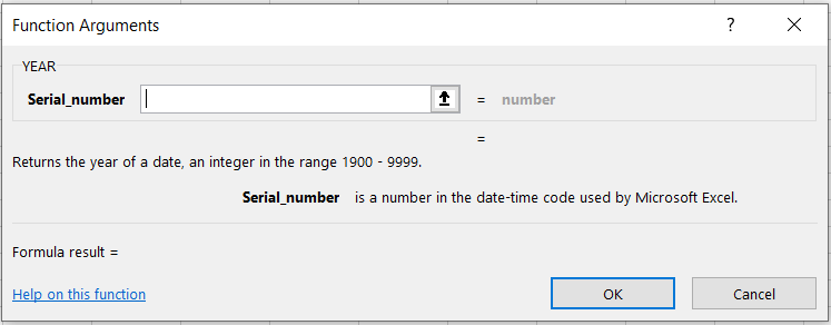
You can use the function in two ways - either from the functions library or as a worksheet formula.

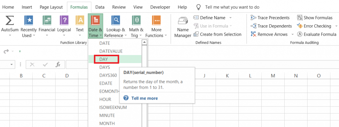
To use the function from the library, click on Formulas > Date & Time and select YEAR from the drop-down menu. 

This will open up the dialog box where you need to input the date as a serial number or directly reference the cell containing the date.

The other method uses the function as a worksheet formula where you begin with the equal sign(=), type in the function name, followed by the argument in the selected cell.

How does the YEAR function work?

To understand how the function works with different date formats, we have illustrated several date formats you will often see in Excel.

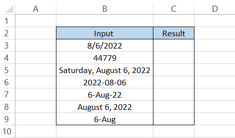
Even though the date is 6th August 2022, it is represented in different formats using the format cell dialog box.

The formula we will use to extract the year component from the dates is =YEAR(B3) in cell C3, which gives us the result of 2022. Then, after dragging down the formula up to cell C9, we get the result:

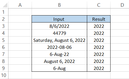
As you can see, even though the formats are different, we get the same result, i.e., 2022. 

Such errors occur when your system has a different date and time format while you input an extra time and date format.

The DATE function takes in three arguments - year, month, and date in the same order. So, for example, if you need to input the date as 6th August 2022, then the formula will be =DATE(2022,08,06) which should give you the expected result.

Examples YEAR Function

Assume that you have a portfolio of bonds expiring in different years. All of them are 10-year treasury bonds paying an annual coupon payment. The date of purchase and maturity are as illustrated below:

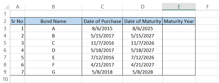
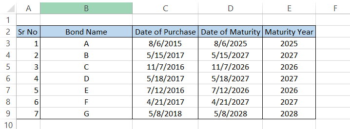
We need to group the bonds according to the year they mature. The formula in the cell E3 will be =YEAR(D3), which will give the result 2025.

After dragging down the formula, we get the result:

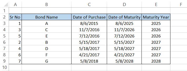
So the only question to be resolved is - how do you get the summary table?

You can select the E column and sort the data in ascending order so that all the bonds maturing in the same year are grouped. 

Press the keyboard shortcut of Alt + H + S + S, which gives you the result:

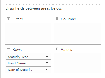
Creating a pivot table is another way of getting precise summary tables. Select the entire table > click on Insert > Pivot Table.

Drag the fields in the PivotTable fields as below:

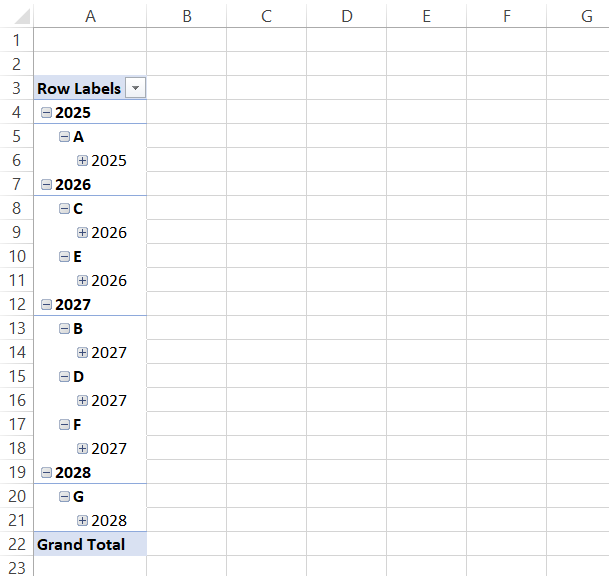
Initially, you would see the pivot table as something similar to this.

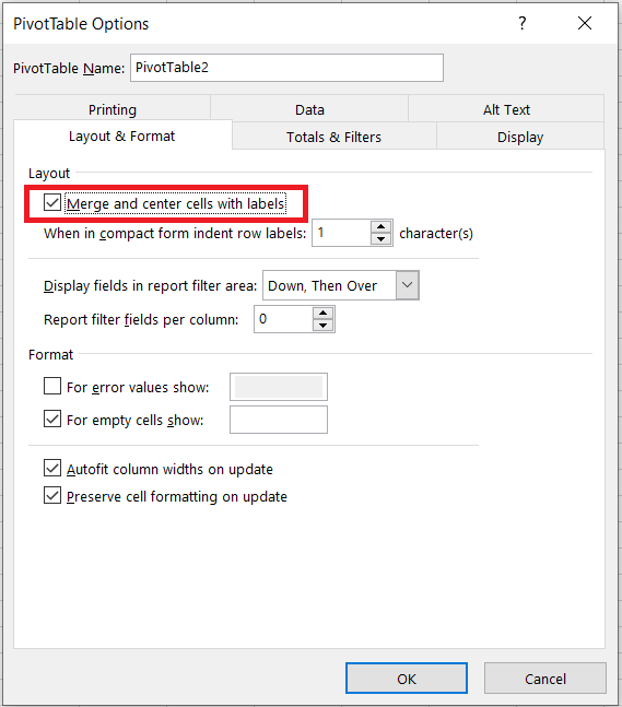
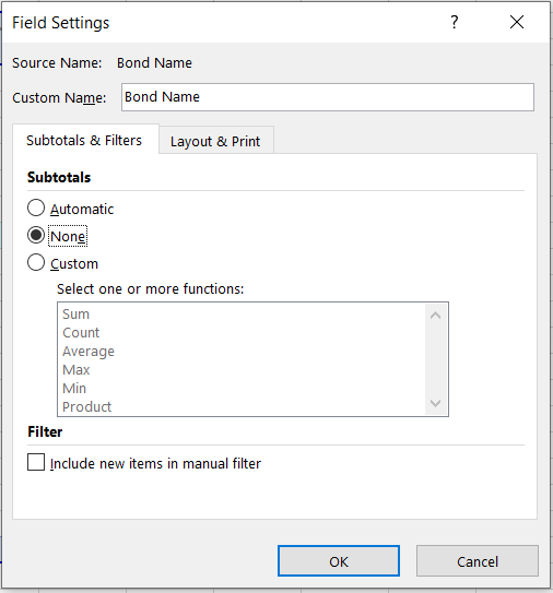
This table doesn't make that much sense. Right-click on table > Pivot table options > and select the 'Merge and center cells with labels.

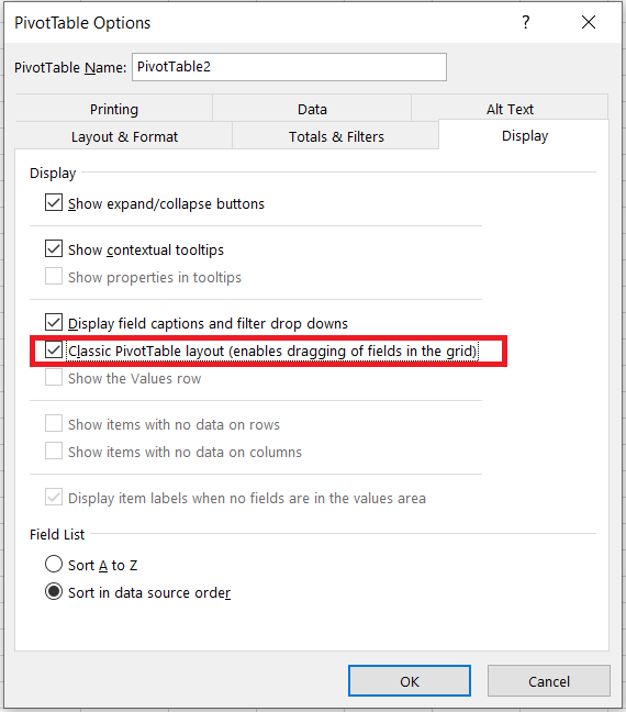
Another change you need to make in 'Display' is to select the Classic PivotTable layout(enables dragging of fields in the grid)

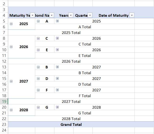
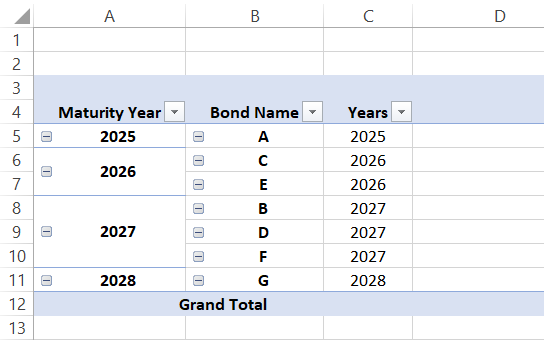
This will change the layout of the pivot table as illustrated below:

You can remove the ‘2025 Total' or 'A Total' by right click on those cell > field settings > Subtotals as 'None.'

After clicking on OK, the final pivot table will look as illustrated below:

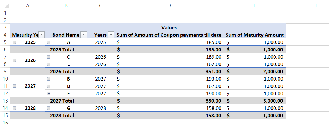
If your table also has two additional columns, 'Amount of Coupon payments till date' and 'Maturity Amount,' then the pivot table can easily accommodate those fields and return the sum of those numbers as a subtotal.

This way, you can know what amount you can expect in a particular year after the maturity of bonds.

Rather than the pivot table, you can also use the SUMIF function to calculate the coupon payments for the bonds expiring in a particular year.

Suppose the data looks as illustrated below, and we need to find the number of coupon payments made for bonds expiring in 2027.

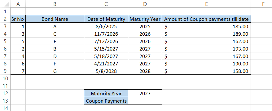
Here, we will use the formula =SUMIF(D3:D9, D12, E3:E9), giving us a value of $550.00.

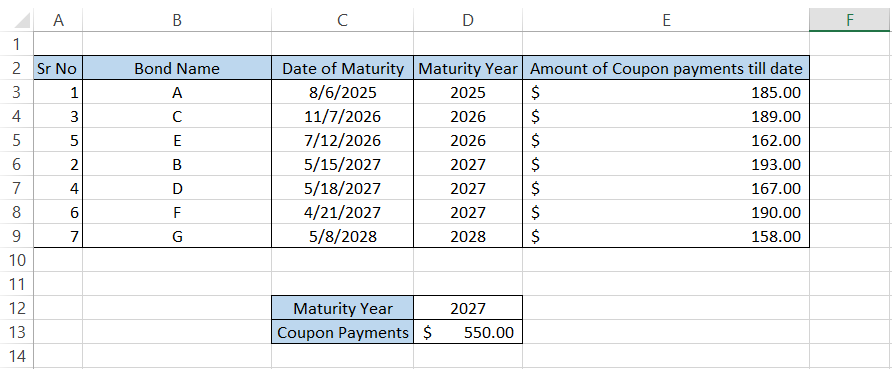
An alternate formula you can also use is =SUMIF(D3:D9, YEAR(C6), E3:E9), which should give you the same result.

The trick is to use the YEAR function and then reference the MM-DD-YYYY for which you want to find the total coupon payments. The extracted YYYY acts as criteria and finds all the values corresponding to 2027 in the range, returning our total coupon payments.

YEAR vs. DAY function

The DAY function returns a number between 1 to 31 depending on the date that you input in the function.

The syntax for the DAY function is:

=DAY(serial_number)

where,

• serial_number = (required) a serial number, the cell containing the date, or a formula that returns the date which will be used to extract the day.

We all own a credit card for shopping and other personal use. However, the amount charged on the card must be repaid to the lender within the due date.

If you have the statements for the credit card in Excel, you can quickly determine whether the due amount is paid within the due date. 

Suppose that the due date is the 5th of every month. If the amount is paid past the due date, the lender charges a penalty of $5 one day after the payment date. The hypothetical credit card statement is as illustrated below:

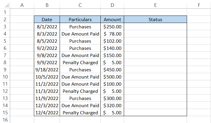
The particulars that need special attention in our statement are 'Penalty Charged.' 

To find if the penalty is levied only if the payments are made after the due date, we will use the formula =IF(AND(C3=" Penalty Charged," DAY(B3)<6), "Unnecessary Penalty levied," "") which gives us the result:

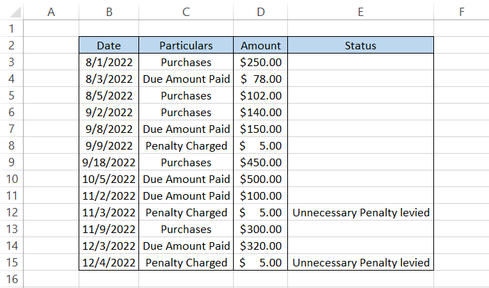
In two instances, we see that the penalty was wrongly charged even though we paid the amount before the due date.

How does the function work?

We input two conditions in the function, both of which must be fulfilled.

• Firstly, the text string in column C must be equal to 'Penalty Charged.'

• The day should be less than 6, obtained using the DAY function.

You must be wondering why the date must be less than 6. Well, the 5th of every month is the last acceptable payment date. Anything after that automatically gets a penalty charge of $5.

When both conditions are fulfilled, we get the result of an unnecessary penalty levied, which can then further be escalated to concerned authorities.

YEAR vs. MONTH function

The MONTH function returns a number between 1 to 12, representing the 12 months from January to December in a particular year.

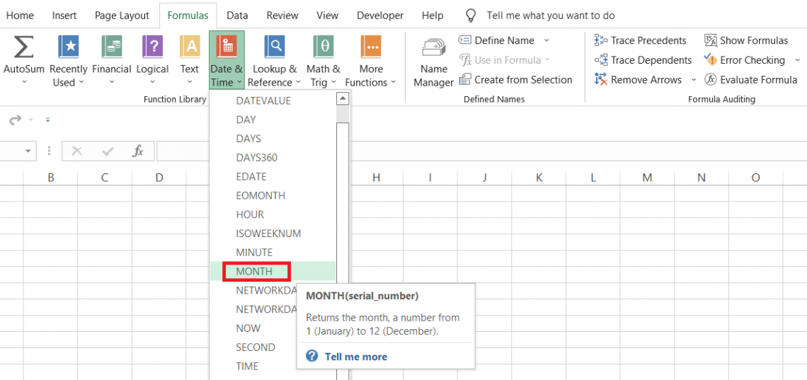
The syntax for the MONTH function is:

=MONTH(serial_number)

where,

• serial_number - (required) a serial number, the cell containing the date, or a formula that returns the date which will be used to extract the month.

Assume that you have a portfolio of ten stocks. The dividend data looks as illustrated below:

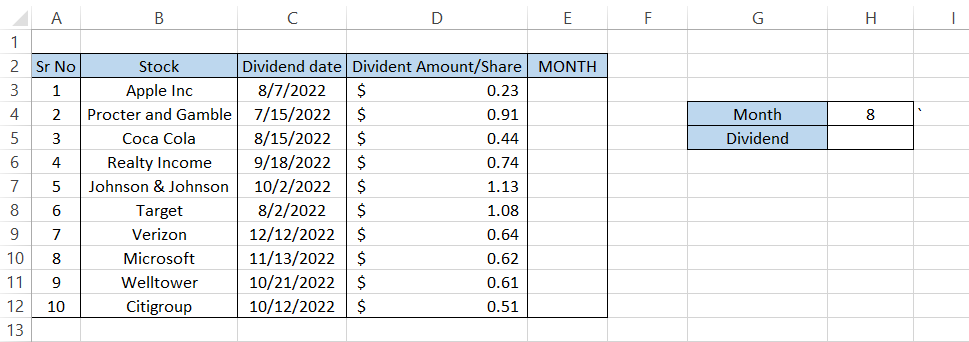
Let's say we only want to calculate the dividend earned in August. We will use the SUMIF and MONTH functions to get the total dividend amount.

First, we will use the MONTH function such that the formula is =MONTH(C3) in cell E3 and drag it down to the last cell, which gives the result:

Next, we will use the formula =SUMIF(E3:E12, H4, D3:D12) in cell H5, giving the $1.75.

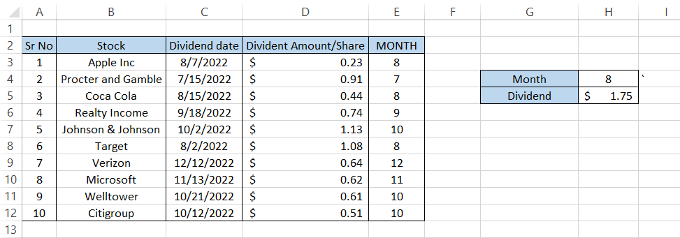
Thus, the total dividend earned in August is equal to $1.75

Researched and Authored by Akash Bagul | Linkedin

Reviewed and edited by Parul Gupta | LinkedIn

Free Resources

To continue learning and advancing your career, check out these additional helpful WSO resources:

• FV Function
• PEARSON Function
• SEARCH Function
• SUBTOTAL Function
• YIELD Function