FALSE Function

What Is The FALSE Function?

A FALSE function in Excel is a Logical Function that returns the boolean value FALSE as a result when used in a blank cell. It is utilized by users as a compatibility function for checking its consistency with other spreadsheet programs

By nature, logical and conditional functions work great in combination with other logical functions such as IF, AND, OR, etc.

If you compare the function's library of Excel to music, we believe logical functions are similar to the Rock genre. They are the soul and spirit of the Excel community since no one could imagine their life without them.

I love Rock 'AND' Roll - Joan Jett & the Blackhearts, Should I Stay 'OR' Should I Go? - The Clash, 'IF' Only - Queens of Stone Age are some of the bangers without which we can't start our day, and the camouflaged functions without which we wouldn't be able to end office hours early.

The idea behind conditional statements is that Excel returns the result as TRUE or FALSE. When the condition is met, the result is returned as TRUE, or it returns as FALSE.

However, using the FALSE function in those statements would work similarly to the NOT function. For example, when you say NOT(TRUE), the function returns the result as FALSE, i.e., the opposite of the logical value.

Similarly, when you input a condition, say 1 > 2 = FALSE, whatever custom text we have assigned for the value_if_true argument will be the result rather than the value_if_false argument. 

This article will help you understand the function's syntax, how to use it, and the various scenarios in which you can 'rarely' use it.

Understanding The FALSE function

The FALSE is categorized as a logical function that returns the boolean value the same as the function's name.

If you have used a lot of conditional statements, you might know that we can just directly input the boolean values as text strings, and Excel would still display the correct result.

So why do we even need a dedicated function?

Since there are many other spreadsheet programs that a person might use based on availability and functionality, Microsoft wanted reports and data generated in 'those' spreadsheet programs to be compatible with their spreadsheet tool.

In short, Microsoft doesn't want any compatibility issues that could give you errors when you open the spreadsheet in Excel.

The function was introduced in the Excel version 2007 and has been ever-present in all the subsequent versions.

The syntax for the function:

=FALSE()

The function takes no arguments. Instead, you begin with an equal sign, type in the function name, complete the formula with parentheses, and smash the Enter key.

We do this when we say 'writing a function as a worksheet formula'. The result is a boolean value that stores the value equal to zero in Excel. 

The other method is:

• Begin with the equal sign, type in the function name, and hit the enter key. No parenthesis is required.
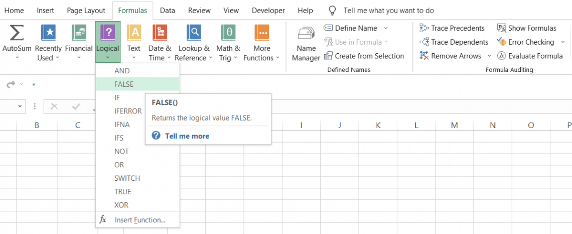
• Click on the Formulas tab > Logical drop-down menu > FALSE

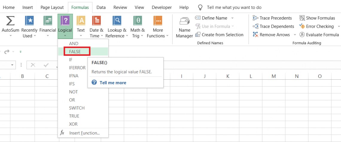
When you click on the function, it will open up the dialog box as illustrated below:

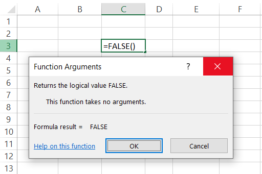
Finally, all you need to do is click on Ok, and the result in cell C3 will be 'FALSE'.

FALSE Function Example

Let's understand how the function works. This section will show examples of how to use the function.

Example #1

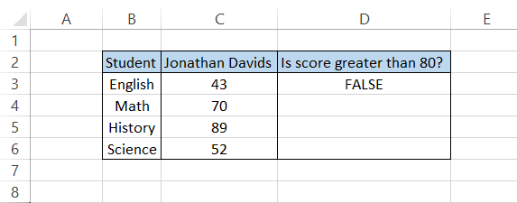
Suppose you must evaluate how many tests Jonathan has scored more than 80. The data looks as illustrated below:

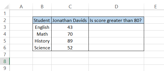
To get the result, we will use the formula =IF(C3>80, "Score is greater than 80",FALSE()) in cell D3, which should give us the result:

Dragging down the exact formula up to D6, the result would be as illustrated below:

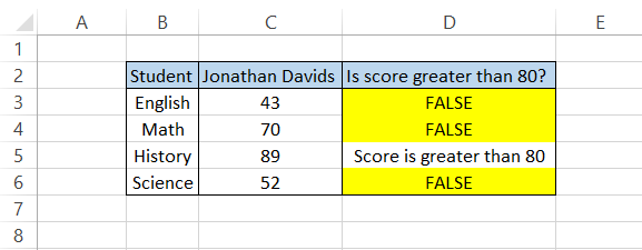
On three different instances, we get the result as 'FALSE' as highlighted in our cells.

Example #2

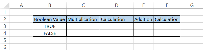
There are two boolean values in Excel - TRUE and FALSE. The former takes in the value of 1, while the latter has a value equal to zero.

We can use this logic to make calculations such as addition or multiplications in Excel.

Let's say we multiply the values in column B by 10. The formula in cell C3 will be =B3*10 which will give us the result as illustrated below:

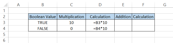
Since TRUE equals 1, when we multiply the function by 10, the result will be similar to the number multiplied. On the other hand, as FALSE stores the value equal to 0, any number multiplied by the function will be equal to zero.

Similarly, when you add a number, say 2, to the function, then we will get the result:

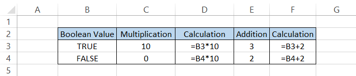
The result for FALSE will always be equal to the number added to the function, whereas for TRUE, it will be one number greater than the numerical value added to the function.

Example #3

Suppose you work for an institutional investor and need to evaluate all the stock holdings in the portfolio. The portfolio looks as illustrated below:

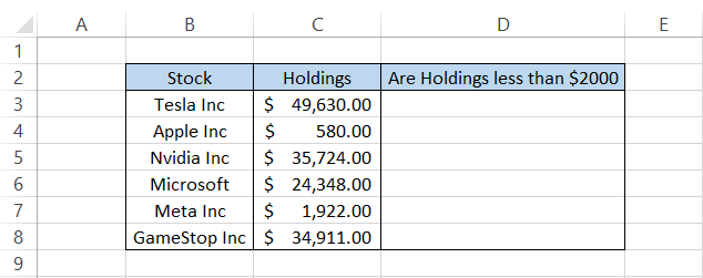
We need to identify what stocks have holdings of less than $2000. For this, we will use the formula =IF(C3>2000,"Holdings are greater than $2000",FALSE()), which will give us the result:

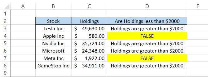
In cells D4 and D7, we get the result as FALSE, where Apple Inc. has a holding of $580 while Meta Inc. has a holding of $1,922, respectively.

Example #4

You can also use the combination of IF, AND, and FALSE functions to evaluate multiple conditions.

Suppose that for the dataset below, we want to match 'Nvidia Inc.' stock purchased for more than $ 171.

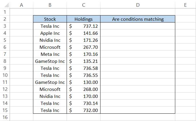
To find a price paid higher than $171 for Nvidia Inc, we will use the formula =IF(AND(B3="Nvidia Inc", C3>171),"Paid higher than $171",FALSE()) which will give us the result as illustrated below:

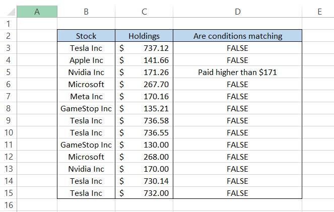
All cells except cell D5 return the result as FALSE since only cell D5 fulfilled both our conditions.

Example #5

If you can use the AND function, then it's pretty obvious you can also use the OR function.

We believe these functions represent the yin and yang of Excel and work great with our compatibility function.

Suppose that you have the marks scored by students in their two different examinations.

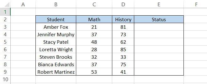
If the student has scored less than 35 in either of the exams, then they must re-appear for the same. 

The formula that we can use to find the status of the students is =IF(OR(C3<35,D3<35),"Re-Appear for Exam",FALSE()), which will give us the result:

We believe you would rarely use this function in your career, but it never hurts to have additional knowledge, right?

TRUE vs. FALSE function

The TRUE function returns the boolean value TRUE while its counterpart returns the boolean value FALSE. We saw that the latter does not have a syntax. Is it the same case with the TRUE function as well?

If you thought yes, then you are right.

The function does not have syntax, and you can use it directly by beginning with an equal sign, followed by the function name, and then ending the formula with the parenthesis.

Again, there are two more methods to use the function:

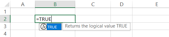
1. In this method, you don't need the parenthesis at the end of the formula. All you need is =TRUE, and press Enter on the keyboard.

2. The other method is from the function's library, where you need to access the function by clicking on the Formulas tab > Logical drop-down menu > TRUE.

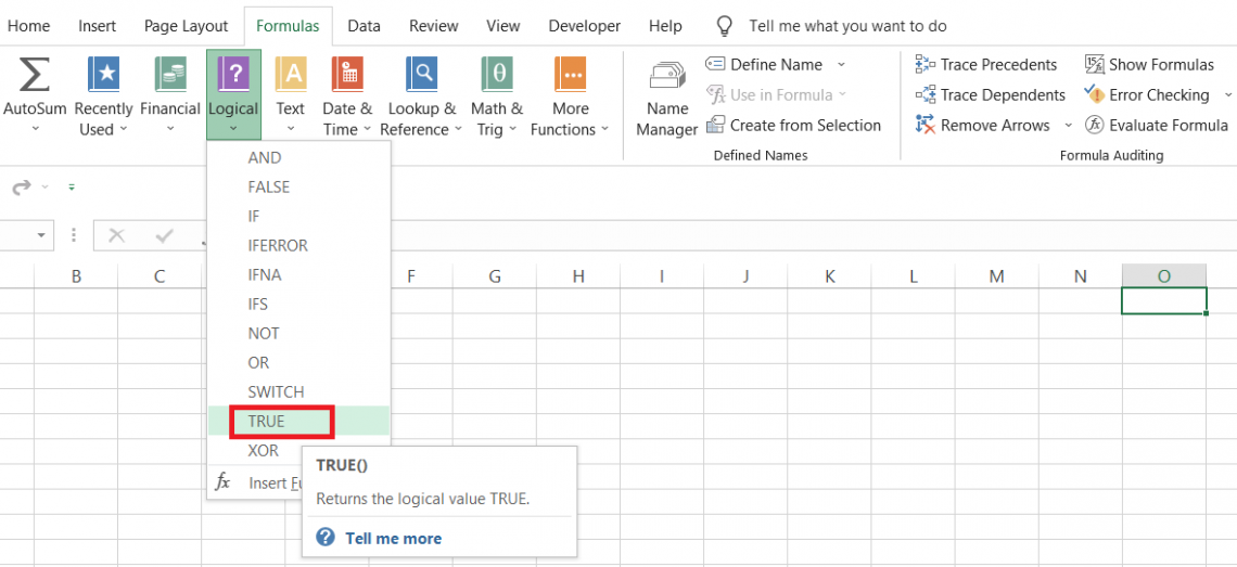
This will open up the dialog box as illustrated below:

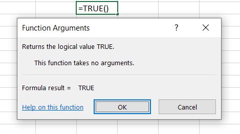
Now, all you need to do is click on Ok, and the selected cell will consist of the boolean value TRUE.

Suppose that you have the examination scores for Mike Byers in different subjects:

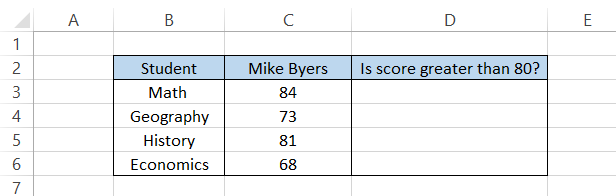
The idea is to determine what scores are higher than 80 and in which subjects Mike scored less than 80.

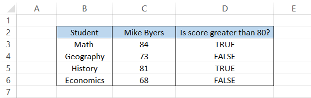
We will use the combination of IF, TRUE, and FALSE functions to find the result. The formula will be =IF(C3>80,TRUE(),FALSE()) which will give the result as:

If you use the TRUE function along with NOT, Excel will return the result as FALSE wherever the condition is fulfilled.

Let's say we want to find all the subjects with scores greater than 80 in the same dataset.

We can twist the formula by including the NOT function so that the formula becomes =IF(NOT(C3<80),"Greater than 80",FALSE()) which will give the result:

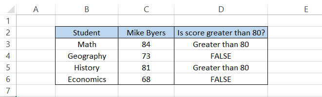
The two significant changes we made in the formula include the NOT function and flipping the comparison operator to less than (<), which gives us our result.

Free Resources

To continue learning and advancing your career, check out these additional helpful WSO resources:

• FREQUENCY Function
• LEN Function
• SUBTOTAL Function
• TIME Function
• TRUE Function