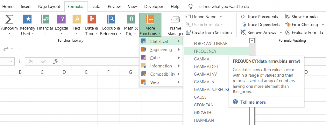
FREQUENCY Function
A Statistical function in Excel that lets you count the number of times an event occurs or a value falls within a user-defined interval range.


What Is The FREQUENCY Function?
The FREQUENCY function is a Statistical function in Excel that lets you count the number of times an event occurs, or a value falls within a user-defined interval range.
For example, a teacher categorizes students into various grades based on their percentage in examinations, different age groups present at a function, etc.
The function's count for recurring events or values can be represented in a visual representation, such as a histogram, to observe patterns in the data, such as which interval had the maximum recurrence. In contrast, you can also determine at what interval the value occurred the fewest times.
As a financial analyst, mastery of this function can help you improve the data analysis and aid in financial modeling.
In this article, we will see how to use the FREQUENCY function in Excel and add it to your arsenal on your way to becoming an Excel wizard.
- The FREQUENCY function is a Statistical Excel Function that is used to analyze the distribution of data values into specified bins or intervals.
- Users provide two arguments to the FREQUENCY function: an array of data values and an array of bin boundaries (or intervals). The function returns an array of frequencies corresponding to the number of values falling within each bin.
- The function aids in statistical analysis by providing insights into the distribution and variability of data values, enabling users to identify patterns, trends, and outliers in their data.
- FREQUENCY function results can be integrated into charting tools to create dynamic histograms and frequency distributions, enhancing the visual representation and interpretation of data.
Understanding FREQUENCY Function
The FREQUENCY is categorized as a Statistical function that returns the frequency distribution for a given list of observations or values.
For example, assume that you have the values as (1,1,1,1,2,2,2,2,3,3,3). If you examine the numbers closely, you will find that the recurrence of the numerical value 1 is equal to four times, 2 occurs four times, while 3 appears three times.
What you did here was visually group all the values under those numbers and return their frequency count. However, you don't need to keep an eye on the numbers while using the function.
Excel does everything for you, from analyzing the numbers for recurring digits to returning the frequency distribution for the values. The function will ultimately return a vertical array of numbers based on the range of intervals upon which it groups the values.
The syntax for the FREQUENCY function:
=FREQUENCY(data_array, bins_array)
where,
- data_array = range of values for which we need to calculate the recurrence
- bins_array = the range of intervals to check the occurrence of values from data_array
Even though the function is relatively easy to understand, many Excel users find it difficult to use. For example, one of the most common problems even Level 78 Excel wizards might run into is that the FREQUENCY function does not return the frequency of the complete data.
There is a high probability that you would get the result only in a single cell despite having multiple values for bin_array.
If you are getting a similar result, there is one big mistake that you are making while using the function. In the next section, we will explore how to 'properly' use the FREQUENCY function and get the desired frequency distribution table for the dataset.

How To Use the FREQUENCY function
If you have tried using the function to return a frequency distribution table, you might not have gotten the expected result on the first try. Well, nobody does when they work on the FREQUENCY function.
If you use the Excel 365 version, the function will automatically return an array of numbers as 'spills,' which isn't the same case with Excel 2019 and prior versions.
This 'how to guide is for those Excel users who work in Excel 2019 and prior versions. The steps that you need to follow are:
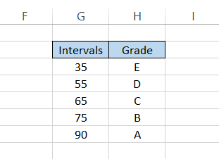
Step 1: Prepare the bins_array or intervals
Before using the function, you must first prepare the range of intervals to group the values in 'those' intervals.
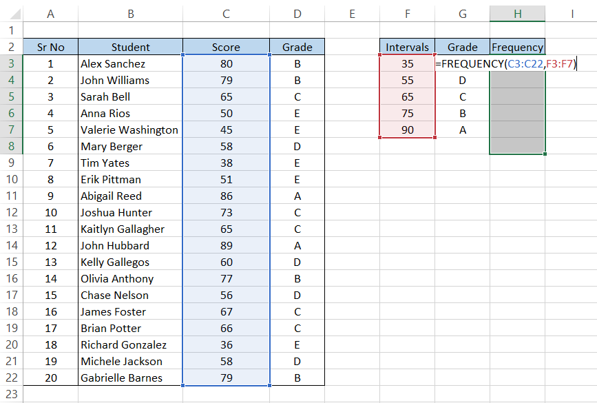
Assume that you have the dataset for a group of students that you need to group into five different grades based on the marks they have obtained in their examination. The data looks as illustrated below:
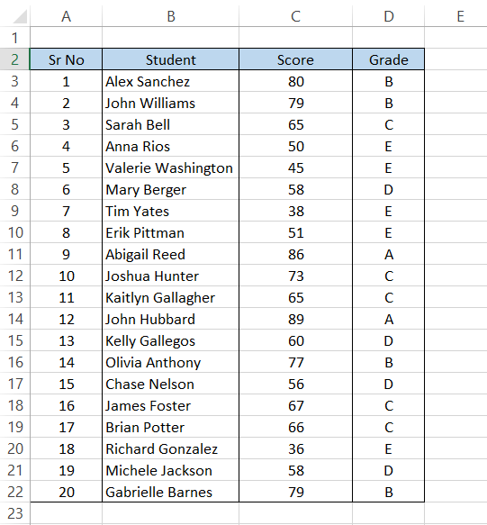
The interval range or the bin_arrays created based on the test scores each student has secured in their examination are :
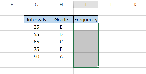
Step 2: Select the range adjacent to bins_array
In the next step, we directly jump to using the formula in Excel. You might have noticed that our intervals in the spreadsheet exist from range G3:G7 (a total of five cells). In addition to those intervals, we have also mentioned the grades in column H.
The most crucial step, in our opinion, before adding the equal sign(=) and FREQUENCY is selecting the range adjacent to our interval's range. In this case, we will choose the range I3:I7.
If our intervals exist in seven different cells, we will select adjacent seven cells before calculating the frequency.
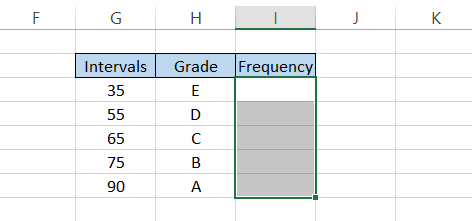
One of the good practices that you can follow is the selection of one additional cell before using the formula. So if the intervals exist in 10 cells on our spreadsheet, we will highlight eleven cells simulating the equation x = y + 1.
Step 3: Use the formula
With the cells highlighted, type in the formula =FREQUENCY(C3:C22,F3:F7) in the first cell of the selected range as illustrated below:
Step 4 : Press Ctrl + Shift + Enter
The final and probably the second most crucial step to display your result is to press Ctrl + Shift + Enter since what you have typed is an array formula.
If you don't press those magic keys, Excel will return the result as zero (that is Excel's way of mocking you for your knowledge about how to use the function).
Once done, the result that the formula should return in Excel is as illustrated below:
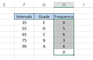
If you check the sum of the frequencies in column H, it will equal the number of observations (scores) we input into our spreadsheet.
We know you are wondering why we selected one additional cell before using the function. The extra cell captures any value that falls outside the largest interval in our bin_array.
For example, if we had a score of 120 in any of the cells, the value would change from zero to one, while the prior recurrence counts would also change.
Example of the FREQUENCY Function
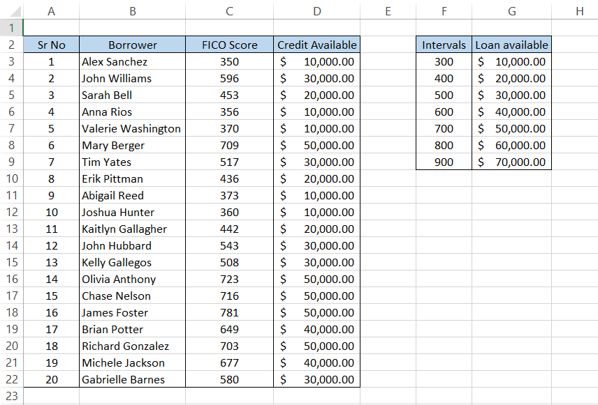
Let's assume that you work at a bank that offers loans to its customers based on the FICO scores that the borrowers have.
A FICO score is a credit score used to screen applicants and other details to assess the credit risk and determine whether the borrower can fulfill their loan obligations.
If the credit score is between 0 and 300, the borrower can qualify for loans worth $10,000. If the score is between 300 and 400, the borrower can qualify for loans worth $20,000.
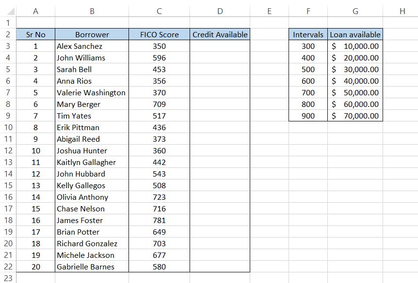
Using the VLOOKUP function, we will pull in the loan available for each person in column D. We will use the formula =VLOOKUP(C3,$F$2:$G$9,2,TRUE) wherein the range_lookup argument as TRUE will find an approximate match for our lookup_value as:
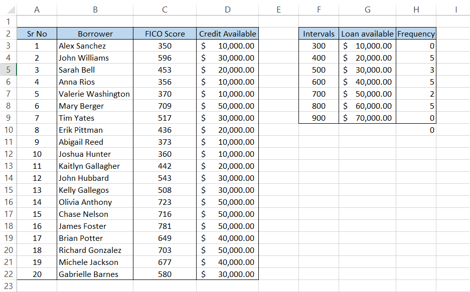
Next, we select the range H3:H9 and type in the formula =FREQUENCY(C3:C22,F3:F9) and press Ctrl + Shift + Enter, which will give us the result in Excel as illustrated below:
Though the chances of Excel creating the wrong frequency distribution table are the same as if you were dating Brad Pitt if you weren't an actress, we can still affirm whether the frequencies returned are accurate using the conditional formatting tool.
The steps you need to follow are:
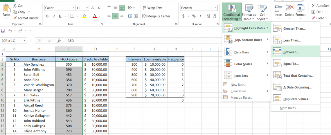
- Let's check whether the recurrence for range 400 equal to five is correct or wrong.
- Select the range, i.e., C1:C22, and then click on Conditional Formatting > Highlight Cells Rules > Between.
- You can also additionally use the keyboard shortcut key of Alt + H + L + H + B to open the 'Between' dialogue box.
4. The values that we will input for 'BETWEEN' would be the previous interval and our current interval, i.e., 300-400, for which we will get highlighted cells as illustrated below:
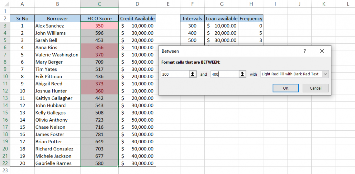
Similarly, you can also check the recurrence for other intervals and find that the count exactly matches what Excel has returned using the FREQUENCY function.
FREQUENCY Function Practical Example
One of the most important reasons to use the function is to create histograms in Excel.
There are other methods, such as pivot tables or the Data Analysis ToolPak but the histograms built using the FREQUENCY function allow more versatility.
The first question that must have sprung to your mind is: Why even build histograms? The most straightforward answer we can think of is that it helps us quickly understand how the data is distributed.
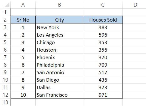
Assume that you have the dataset for houses sold in some of the US cities as illustrated below:
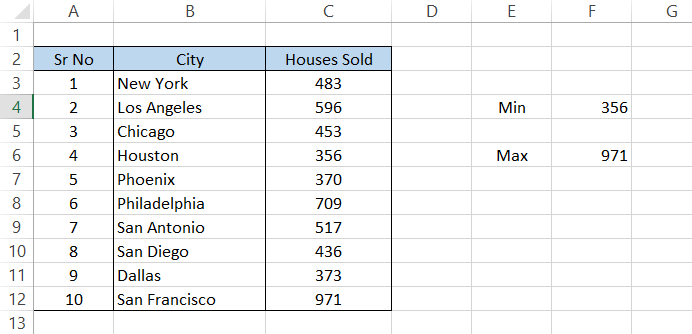
We will first create the bin_array of intervals which is also a prerequisite for creating a histogram. We usually find the minimum and maximum values using the MIN and MAX functions, respectively and then make the intervals.
The formula will be =MIN(C3:C12) and =MIN(C3:C12) in cells F4 and F6, respectively, which will give us the result:
It makes sense to start bin_array from 350 to 1150 with an interval of 100. So far, the spreadsheet looks as illustrated below:
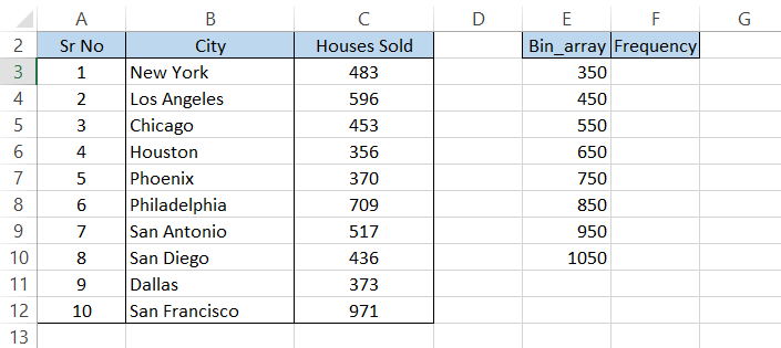
The next step is easy! Select the range F3:F11 and type in the formula =FREQUENCY(C3:C12,E3:E10), which will give you the frequencies of the house sold.

Finally, we plot the graph using the data available, i.e., the bin_array and the frequency. Select the data > Click on Insert > Charts > 2-D Column charts. Once you make all the customizations, the histogram should look as:
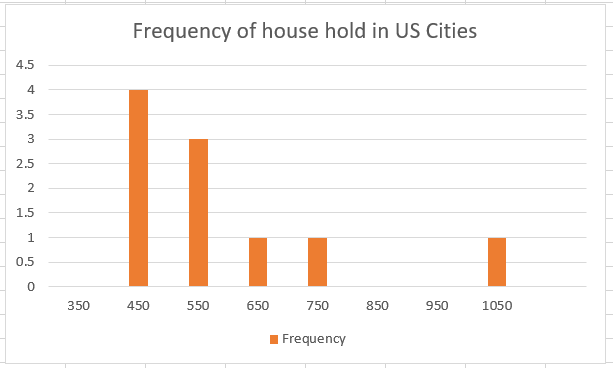
The histogram helps us to interpret that in most US cities in our data, four have sold between 350-450 houses, three cities sold between 450-550, and the rest of the three cities sold homes ranging between 550-650,650-750 and 950-1050, respectively.
Summary
- The FREQUENCY function will return the count for the recurrence of a value in a dataset.
- An important thing to remember is to select the range of cells in which you want the frequency table. If you do not input the reference to an empty range of cells, you will most likely get an incorrect result.
- If you reference a range of cells that contains a text value or is empty, the function will ignore such cells in its result.
- If the referenced data_array does not contain any numerical values, Excel will return the result for the formula as zero.
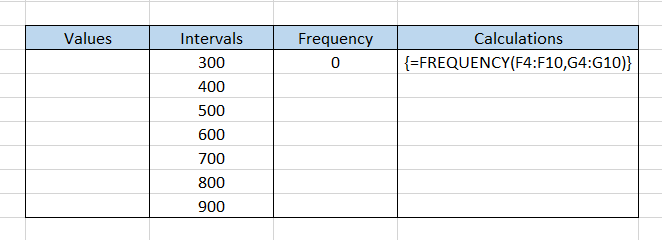
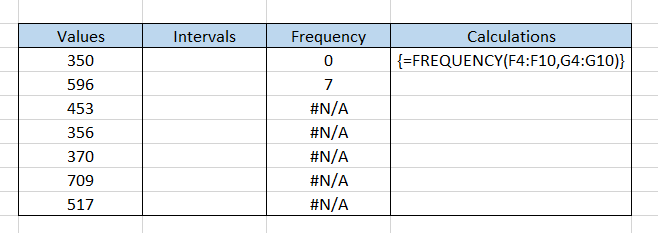
- If the referenced bin_array does not contain the intervals, then Excel will return the result equal to the number of elements in data_array. For example, if data_array has seven elements, the result would equal 7.
You will see that additionally, the formula also results in #N/A errors in Excel.

Free Resources
To continue learning and advancing your career, check out these additional helpful WSO resources:


or Want to Sign up with your social account?