PMT Function
An Excel Financial Function that is utilized to calculate the periodic payments of loans, taking fixed interest rates and a number of payments into consideration.


What is the PMT Function?
PMT function is an Excel Financial Function that is utilized to calculate the periodic payments of loans, taking fixed interest rates and a number of payments into consideration.
PMT function is a traditional financial Excel function prominently used in various settings. For example, it can calculate the necessary payment to fulfill a loan obligation, payment in annuities, or investment returns with a fixed interest rate over a specified period.
While using the function assumes that the problem it is trying to solve has some sort of consistent and periodic cash outflow, a constant interest rate throughout the period, and the total number of periods used to make the payments.
The function makes users more convenient and less time-consuming to calculate the loan or mortgage obligation with a simplified form. Users may use the calculator to grasp an approximate amount of payment needed to fulfill their obligation before committing to one.
The acronym used for this function, “PMT,” comes from the word “payment,” which exemplifies the function’s name. As the function’s name, it helps calculate the payer’s negative amount, hence the payment outflows from the cash amount.
The payment amount calculated using the function only includes the principal and consideration of the interest rate. It does not include additional fees, taxes, or other circumstances beyond the principal amount, interest rate, or payment periods.
Learning how to use the function can simplify your life by easily calculating the amount of repayment toward loans, mortgages, or annuities. These financial instruments have different payment frequencies, including weekly, monthly, or even annual intervals.
At this time, the function is available in most Excel systems, including
- Excel 2007
- Excel 2010
- Excel 2013
- Excel 2016
- Excel 2019.
- The PMT function is an Excel Financial Function that is used to calculate the periodic payment for a loan or investment based on constant payments and a constant interest rate.
- The PMT function calculates the periodic payment (such as monthly or annual) required to pay off a loan or investment over a specified period, given a constant interest rate and constant payments.
- The PMT function requires numerical values for its arguments. If any of the input arguments are non-numeric or invalid, it may return an error.
- The PMT function may return an error if the specified interest rate or a number of periods is outside the valid range or if any of the input arguments are invalid. In such cases, it may return a #NUM! or #VALUE! error indicating the nature of the problem.
PMT Function Formula
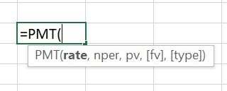
= PMT(rate, nper, pv, [fv], [type])
- Rate (required) - refers to a constant or fixed interest rate
- Nper (required) - refers to the payment period, specifically the “number of payments” that are needed to be made for the entire obligation
- PV (required) - is an acronym for present value or principal value and usually refers to the total loan or annuity amount
- FV (optional) - is an acronym for future value and usually refers to the goal amount at the end of obligation - for loans and mortgages, FV should be 0
- Type (optional) - a boolean section with a binary feature indicating when the payments are due by either 0 or 1;
- 0 = end of period, 1 = beginning of period.
- If you keep this blank, the default will automatically set it to 0 at - the end of the period.
All required values must be inputted for the function to derive a value. These required values include RATE, NPER, and PV. The optional values are up to you to input in the function to advance or specify a direction. These optional values include FV and TYPE.
How to use the PMT Function in Excel?
The function can be used by typing directly in the cell or finding it through the menus. First, if you are typing the function directly in the cell, you must use the “=” equal sign to indicate the beginning of the function.
- Select a cell to input the value derived from the function
- Start with the equal sign, “=”
- Type as shown under the formula section, the function formula is:
= PMT(rate, nper, pv, [fv], [type]).
4. Note that all the values within the function must be numerical or boolean (typically for the [type]).
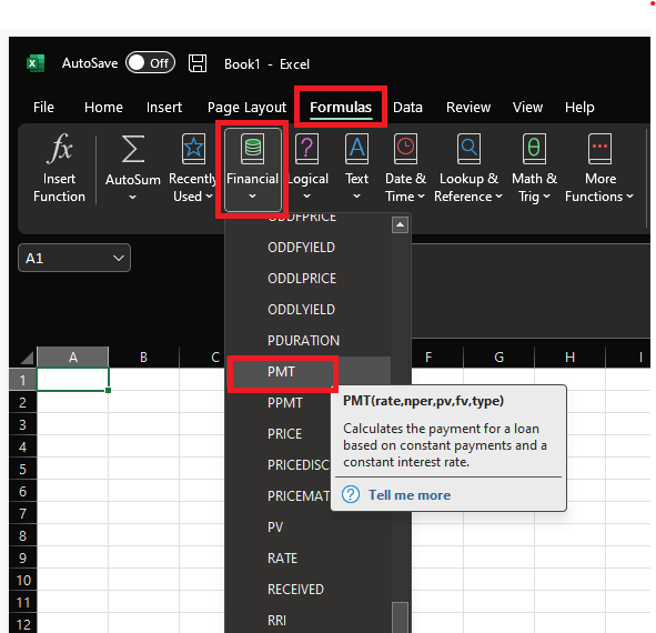
Another way around this is to find the function using the menu tabs in the Excel spreadsheet. You may find the menus shown below.
- Click the Formulas tab at the very top of the Excel spreadsheet.
- Click the “Financial” table below the Formulas tab
- Scroll down and look for the function
PMT Function in Loan or Mortgage Calculation
PMT function can calculate the monthly payment of a loan or mortgage the borrower should repay to their financial institution.
The calculation requires the loan amount, interest rate, and the number of payments made throughout the repayment process.
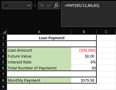
In this example, the present value is the loan amount of $30,000. Note that the loan amount has a negative sign or is negative in value. This is to note that the amount is potentially “used” being drafted out of the lender’s pocket. The future value is to repay the negative balance to $0.
The interest rate will be the rate at which the loan is being borrowed, which is 6% annually. Therefore, the total number of payments is 60 months, assuming that the borrower must repay the loans monthly over the five years: 5 * 12 = 60.
For the loan and mortgage example, the goal is to pay back the $30,000 after 5 years with an annual interest rate of 6%. The formula in cell B8 is:
= PMT (B5/12, B6, B3)
Note that the rate (cell B5) was divided by 12 in the function. This is because the example initially had an annual interest rate of 6%, which should be divided by 12 months per year to match the NPER we used, which is the monthly payment.
Since there are a total of 60 months in this example, the loan of $30,000 can be repaid to the financial institution in 5 years by paying a fixed amount of approximately $580 at the end of every month.
Calculate by Different Frequencies of Payment
| Payment Frequency | Edit in Rate | Edit in Nper |
|---|---|---|
| Weekly | Annual Interest Rate / 52 | Year(s) * 52 |
| Monthly | Annual Interest Rate / 12 | Year(s) * 12 |
| Quarterly | Annual Interest Rate / 4 | Year(s) * 4 |
| Tri-Annually | Annual Interest Rate / 3 | Year(s) * 3 |
| Semi-Annually | Annual Interest Rate / 2 | Year(s) * 20 |
The PMT function can be used to calculate the payment of different frequencies. The table above shows what you must adjust to create those results using the function in Excel. First, the “rate” and “nper” parts of the formula must be adjusted, as shown above.
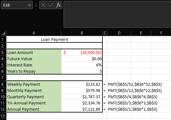
Let’s continue with the above example and say you borrowed a $30,000 loan from a bank with an annual interest rate of 6% and are obligated to pay it back within 5 years. Recalling the function’s formula:
=PMT(rate, nper, pv, [fv])
If the obligation sets you to pay back a partial amount of loans each week, the function will change as shown in the “Weekly Payment” row:
=PMT(0.06/52, 5*52, -$30,000, 0)
Because there is 52 weeks total in a single calendar year, note that the “rate,” which is an annual 6% interest, was divided by 52 weeks. Similarly, since the “nper” indicates the payment period, which is 5 years, it is multiplied by 52 weeks.
Using this function, the result ends up with a $133.62 weekly payment. Similarly, if the loan must be paid back quarterly, the function will change to this:
=PMT(0.06/4, 5*4, -$30,000, 0)
Because quarterly means dividing the calendar year into 4, the rate and nper were adjusted by dividing and multiplying by four, respectively. This then results in a payment of $1,747.37 quarterly or every three months within a year.
PMT Function in Annuities
Annuities are financial products or contracts usually distributed and issued by insurance companies or similar financial institutions that guarantee investors a fixed income stream structure.
Depending on the type of product the investor funds, the annuity product may reimburse the investor with periodic cash flow up to a contracted amount or pay the investor in a lump sum at the end of the contract term.
The annuitant or the investor must pay an obligated monthly or annual premium to keep the contract ongoing. In addition, since the contracts are illiquid, the annuitant may not touch the money during the surrender period.
The surrender period may last from 2 years to more than ten years, depending on which type of product the investor chooses. Surrender fees, also known as penalty fees, could be 10% or more, depending on the contracted product.
The function can calculate the periodic payment or premium the annuitant should pay through the annuities once contracted. The calculation requires the future value, interest rate, and the number of payments made throughout the contract.
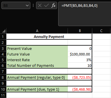
In this example, we have an initial present value of 0 because there is no expenditure in the beginning. The future value is the goal to attain $100,000 at the end of 10 years. The NPER period is ten years, assuming payments will be annually paid. The interest rate is at 3% annually.
For the regular annuity example, the goal is to attain $100,000 after a 10-year period with an annual interest rate of 3%. Assume that annual payments are made at the end of each year for a regular annuity. The formula in cell B8 is:
= PMT (B5, B6, B3, B4, 0)
Note that the 0 at the end denotes the regular annuity with annual payment assumed to be paid at the end of each year.
For the annuity due example, the goal is to attain the same amount of $100,000 after 10 years with an interest rate of 3%. Assume annual payments are made at the beginning of each year for an annuity due. The formula in cell B10 is:
= PMT (B5, B6, B3, B4, 1)
Note that the 1 at the end denotes the annuity due with annual payment assumed to be paid at the beginning of each year.
PMT Function Errors
The PMT Function may contribute to errors and produce wrong results if you misuse them.
There are several errors that you should look out for if you are using the function, and you can troubleshoot them by using these examples:
- #NUM!: The NUM error may occur when you input the wrong information for either RATE or NPER portion of the function. It appears if you input a negative number for the RATE. RATE should never be a negative value. It appears if you input a 0 for NPER. Therefore, NPER should not equal 0 at any point.
- #VALUE!: The VALUE error may occur when you input textual data in any portion of the function. Remember that all the portions of the function are or should be numerical.
- Extremely High or Low Amount: You know you are doing something wrong if the payment amount resulting from the function is in its extreme form, whether it be a low or high amount.
In this case, try to double-check what you have inputted for RATE and NPER. The two values may not be aligned. For instance, using an annual rate with monthly NPER will result in a lower payment amount.
Another way is to double-check what you might have inputted for RATE. For example, notice that if you put RATE = 6 intended for a 6% interest, the 6 will stand for 600% interest, not 6%, due to the basics of the whole number.
Summary
PMT Function is utilized to calculate different payments of obligated loans, annuities, or mortgages with a set cash flow of payments with constant interest rates in a specified period.
The function formula is
= PMT(rate, nper, pv, [fv], [type]),
where the rate is the interest rate, nper is the payment period, PV is the principal value, FV is the future value, and type distinguishes the payment made either at the beginning or end of the payment period.
Rate, Nper, and PV are required values to be inputted, while FV and Type are optional to the user to enhance or advance the specification in the function.
All values within the function must be numeric and/or boolean.
The payment returned by this function only incorporates the principal amount (e.g., loan amount) and the interest rate. The calculation does not include additional fees, taxes, or other types of outflows.
Errors can be induced by inputting wrong information into the function. Ensure consistency with the unit in rate and nper, and be aware not to input negative values for rate or nper.
It’s important to input the loan amount as negative at the beginning, indicating that the monthly payment is negative. Again, aligning with how you want to express your values and interests is important.

Free Resources
To continue learning and advancing your career, check out these additional helpful WSO resources:


or Want to Sign up with your social account?