CHOOSE Function

What is the CHOOSE Function?

The CHOOSE function allows us to return an item on a list when we input an index number that corresponds to the item

Let’s try to create an analogy to understand the function better. What do you do when you are hungry? You go to the nearest McDonald’s. You decide to get a combo meal for yourself - 2 cheeseburgers with medium fries and a medium coke.

However, in today’s fast-paced world, no one has the time to make all those descriptions (except when you want the pickles or not), and neither do the cars in the queue behind you. 

You just say to the person in charge,” Can I please get one number 9 to go?” And that is the end of it. By the time you reach the pickup window, your food is already waiting for you, i.e., two cheeseburgers with medium fries and a coke. What happened here?

We see that, based on the ‘index number’ for the combo meal on the menu, you decide to order a specific food item. 

Of course, you always describe how you want the food to be made, but the general idea is that a unique number corresponds to a particular food item on the menu.

It works in the same way, where we input the index number that will then check the values that fall under that index number and return the result in the spreadsheet.

Understanding the CHOOSE function

The function is categorized as a Lookup and Reference function that returns a value from the specified list based on the index number inputted.

For example, if you have three different fruits on a list, apples, mangoes, and pineapples, and use the index number as 2, the result will be “mangoes” since it is the second fruit on the list.

You can use the function to return different values based on the index number.

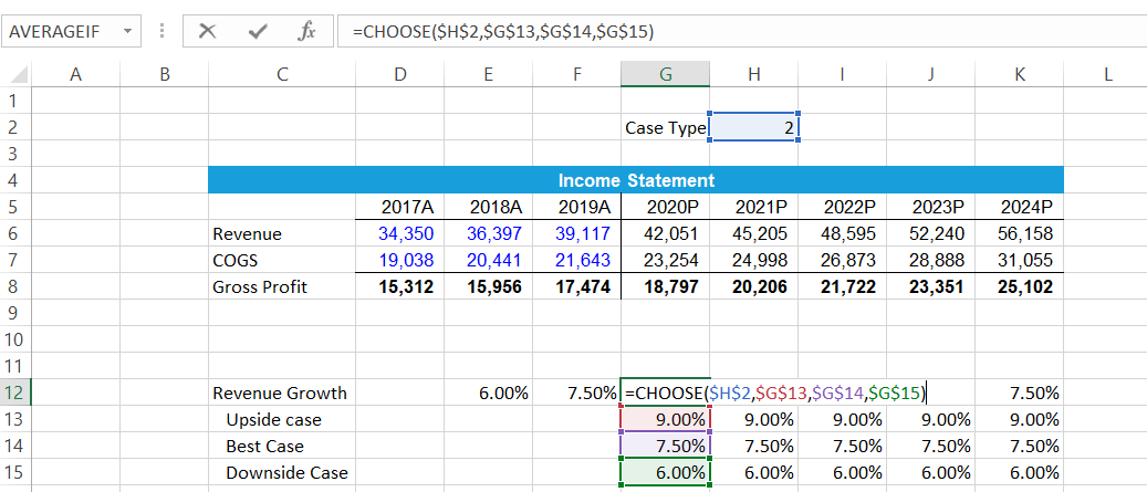
For example, when preparing financial models, you can use this function to set up the different financial drivers, such as revenue growth for the upside, base, and downside cases. 

By changing the case type (index number) between 1-3, the financial model will reflect the change in the financial model and the revenue earned when the revenue growth differs for different scenarios. 

This is just one way you can show the changes in financial drivers.

Check out our Financial Modeling Course, where you will learn how to prepare a Nike model from scratch!

CHOOSE function Formula

When we talk about the capabilities of the function, let's just agree the function looks straightforward. 

We have all found Excel functions that were difficult to understand but had a really simple syntax, while, on the other hand, others had a difficult syntax but were quite easy to interpret.

The function falls in neither category and has a distinct personality.

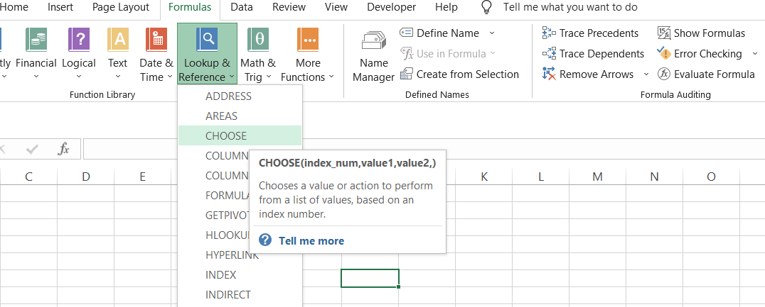
The syntax for the function is:

=CHOOSE(index_num,value1,[value2],..)

where,

• index_num = (required) argument used to specify which value to return based on its position.
• value1 = (required) The first value in the list can be returned by using the index_num as 1.
• value2 = (optional) The second value in the list that can be returned by using the index_num as 2.

You can input up to 254 values in the function and index them based on the value between 1-254.

The value in the function can be a number, text string, cell reference, or even a formula cell. However, if you reference a range of cells directly, you might get a #VALUE! Error.

How to use the CHOOSE Function in Excel?

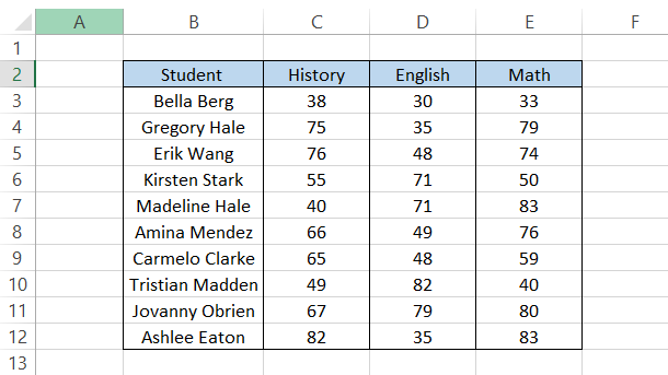
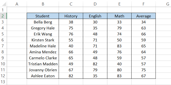
Assume that you need to find the grade scored by a student based on the average marks in three different subjects - history, math, and English. The data looks as illustrated below:

To find the average and determine the grade in which they fall, we will create an additional column ‘Average’ and derive the mean score of the three subjects using the formula

=AVERAGE(C3:E3)

to give the following result:

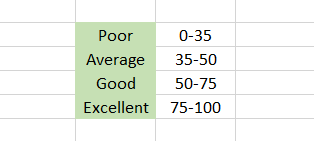
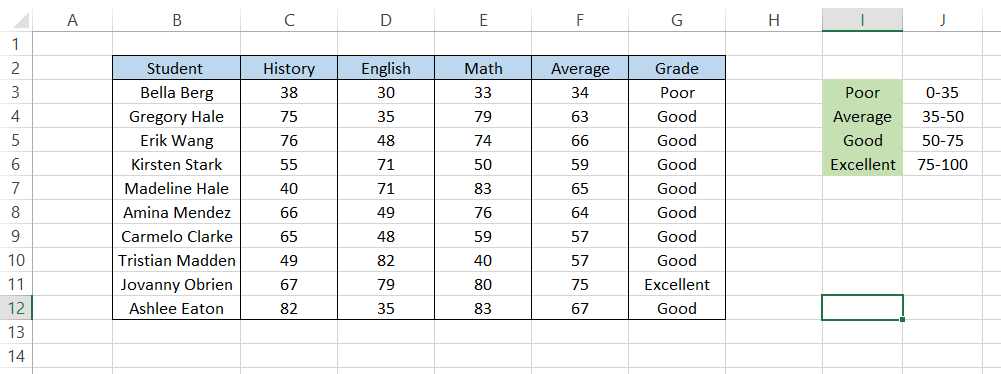
Next, you will use the criteria to assign the grade to the students based on the average score in column F. The formula that you will use is 

=IF(F3>0,CHOOSE((F3>0)+(F3>35)+(F3>50)+(F3>75),$I$3,$I$4,$I$5,$I$6,)), 

which will give you the results:

We begin with the argument that our average score is greater than zero, which it obviously is. As that condition is fulfilled, we ask Excel to select the value based on the index number. 

The result for the criteria can either be TRUE or FALSE, often represented as 1 and 0 in Excel as well. 

So, if the average of the three subjects is greater than 0, you will get the result of 1. If the average is greater than 35, the result will be 1, and so on. 

All these zeros and ones are then added to the index number, which will finally return the result from the values' Poor, "Average," Good,' or' Excellent.' 

For example, for student Erik Wang, we can see that the average score for all three subjects is 66. 

Hence, it passes as true for the first three criteria in the function: (66>0) + (66>35) + (66>50). However, it doesn't pass the fourth criterion: (66>75), i.e., it is neither greater than nor equal to 75.

Hence, the index number that forms is (1+1+1+0), which is 3. This corresponds to the value in cell I5 in our list, which is 'Good.'

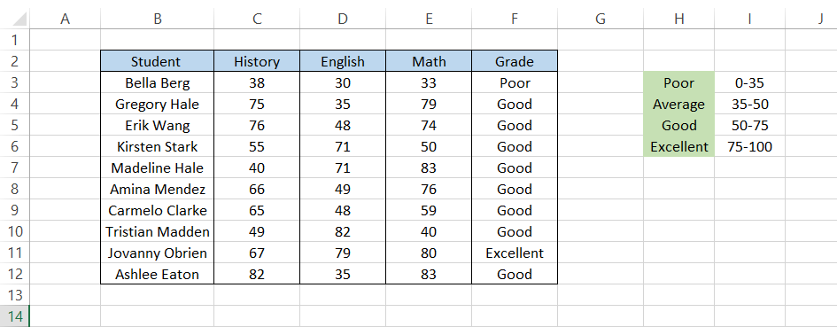
You can also remove the ‘Average’ column from the spreadsheet by using it directly in the formula: 

=IF(AVERAGE(C3:E3)>0,CHOOSE((AVERAGE(C3:E3)>0)+(AVERAGE(C3:E3)>35)+(AVERAGE(C3:E3)>50)+(AVERAGE(C3:E3)>75),$H$3,$H$4,$H$5,$H$6,)) 

This will give you the same result in the spreadsheet but might make things a bit difficult to understand.

There is never any right or wrong in what you do. Just proceed with what you feel most comfortable with.

We have used the AVERAGE function in the formula. This function returns the average value for a range of cells in Excel.

Left lookup using the CHOOSE function

You may already know that you cannot look up a value to the left using the VLOOKUP function in Excel. The alternative uses the combination of INDEX MATCH (or XLOOKUP) that returns the result to the left of the lookup_value. 

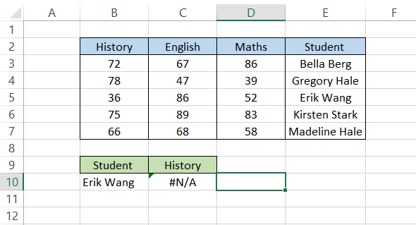
However, there is a loophole that you can exploit to help find a value to the left using the VLOOKUP function: nest the CHOOSE function. Assume that you have the data representing marks scored by students in their exams as illustrated below:

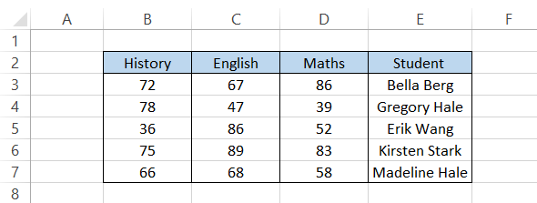
If you need to find the mark scored by Erik Wang in his history test, the formula that you will use is

=VLOOKUP(B10,B3:E7,1,FALSE)

but that doesn't return the result; instead, it gives you an #N/A error.

To avoid the error, you can nest the CHOOSE function inside the VLOOKUP such that the formula becomes 

=VLOOKUP(B10, CHOOSE({1,2,3,4},E3:E7, B3:B7,C3:C7, D3:D7),2,FALSE)

to give you the result as:

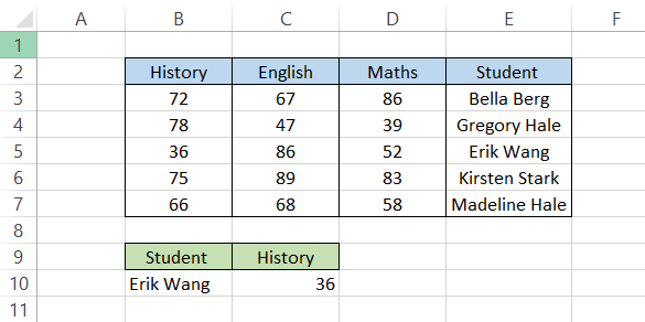
The function rearranges the columns in the formula by assigning the index_num 1 to the Student column while the subject marks for History, English, and Math become index_num 2,3 and 4, respectively. 

This way, even though the data is not properly set up for a left lookup, the inclusion of the CHOOSE function lets you overcome this.

CHOOSE Function Practical Examples

If you are on the path to becoming an Excel wizard, nothing can help you more than reading a lot about different Excel functions and practicing those formulas in spreadsheets.

To help you level up faster, we have brought you more examples. Let’s go! 

Example #1 

Assume that, for the cultural events, you need to divide students into four groups based on their age. The list of students participating in the cultural events is as follows:

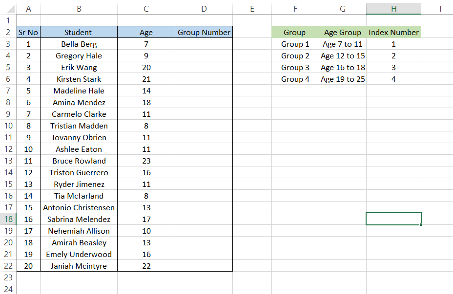
To assign the group number to each student, you will use the formula

=CHOOSE(IFS(C3<=11,$H$3,C3<=15,$H$4,C3<=18,$H$5,C3<=25,$H$6),$F$3,$F$4,$F$5,$F$6)

returning the following result:

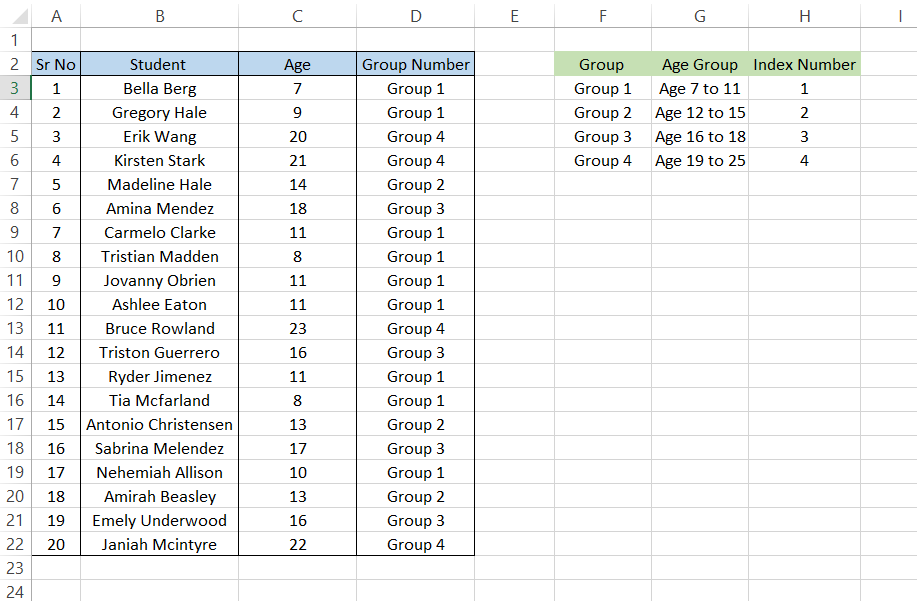
The IFS function checks the age of the student in column C and investigates in which age group it falls. 

For example, if the student falls in the 7 to 11 age group, the index number 1 is taken for further results. If the index number is 1, then the group for the student is returned as ‘Group 1’.

Example #2

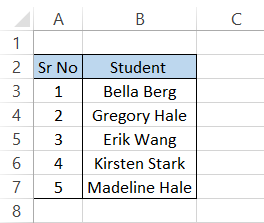
Assume that you need to select a random student from a group of five for the presentation. The five students in the group are:

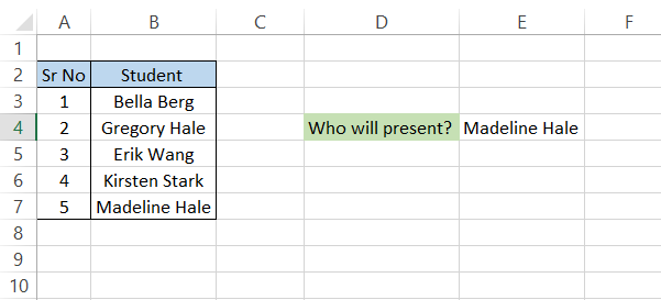
If you want to select a student randomly, you will use the formula 

=CHOOSE(RANDBETWEEN(1,5), B3,B4, B5,B6,B7)

which will give you the result in cell E4 as:

The RANDBETWEEN function returns a random number based on the numerical upper and lower limits. 

For our example, we have set the lower value as 1, while the upper value is 5, i.e., the number of students in the group. 

Since the RANDBETWEEN is a highly volatile function, the value in cell E4 will automatically change whenever you make any changes in the spreadsheet.

This can be fixed by going into the Formula menu in the ribbon, then Calculation Options, and then Manual. This means that nothing will calculate automatically, requiring you to click the F9 key to refresh your workbook for new/updated formulas.

Conclusion

The CHOOSE function in Excel serves as a versatile tool for retrieving specific values from a list based on an index number. Analogous to ordering from a menu at a restaurant, where each item corresponds to a unique number, CHOOSE simplifies data retrieval and manipulation.

CHOOSE function's integration with other Excel functions like IF and RANDBETWEEN expands its utility, allowing for dynamic decision-making processes and randomized selections.

Whether assigning grades based on average scores or randomly selecting candidates for a task, CHOOSE empowers users to streamline their workflows and enhance efficiency.

By understanding its mechanics and exploring practical examples, individuals can leverage CHOOSE to expedite tasks, make informed decisions, and unlock the full potential of their Excel spreadsheets.

Free Resources

To continue learning and advancing your career, check out these additional helpful WSO resources:

• FV Function
• PEARSON Function
• SEARCH Function
• SUBTOTAL Function
• YIELD Function