LEN Function

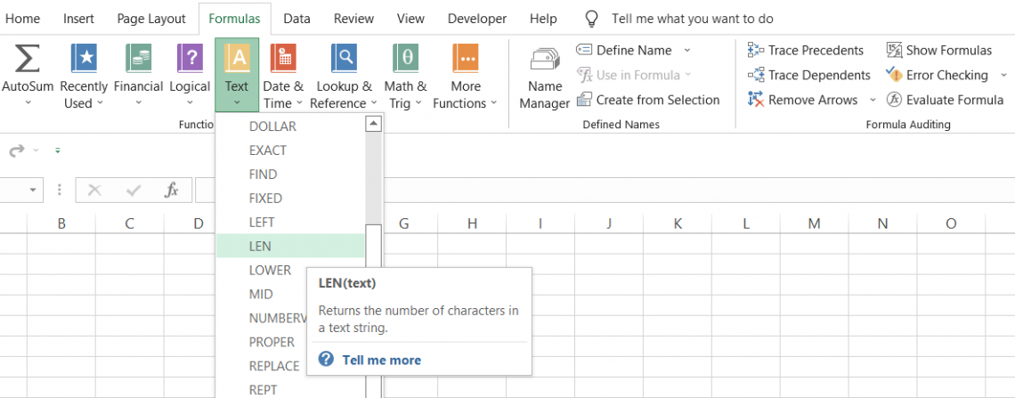
What is the LEN Function?

The LEN function in Excel returns the length of the text string or a numerical value as a whole number. 

As a financial analyst, you often work on data that may consist of unnecessary characters.

To remove those additional characters, a LEN function is used. It helps to determine the string’s length and then cut off the required characters. 

The function generally allows for all types of text manipulations by collaborating with other text functions such as RIGHT, LEFT, MID, etc.

Whether you are working on a task as simple as separating first and last names, counting the number of words in a text string, or as complicated as finding the ‘nth’ word in a sentence, the LEN function plays a pivotal role.

That’s a bit of advanced Excel, which we will get to later. But, first, we shall begin with how the function works as well as the syntax for the function. 

Understanding the LEN Function

The LEN is categorized as a text function that will count the number of characters in a text string. If you use a numerical value, then the function can even count the digits in the numerical value.

For example, if you have the value 928 in Excel, the result returned in the spreadsheet will equal three. Now, count the letters in the word, and you will find it exactly matches our result. Easy right? 

As you can see, Excel does not return an error in the case of numerical function despite LEN being primarily a text function. 

Next, if you have the word ‘WallStreet Oasis,’ the function will return the length of the string as 15. This is because the letter ‘W’ takes the index position as 1 up to the letter’ s,’ which takes the index position of 15.

Based on the final index position value, the function returns a result equal to 15.

LEN Function Formula

The syntax for the function is:

=LEN(text)

where,

text = (required) text string enclosed inside the quotation marks, a cell reference for the text string, or a formula that returns text.

LEN Function Examples

Since the syntax is quite easy to understand, we will head over to an example and see how the function affects different values in Excel. Let’s say you have data in Excel, as illustrated below:

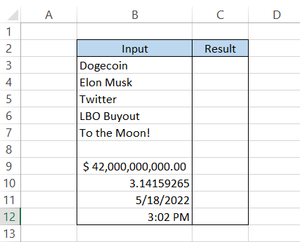
We will use the formula =LEN(B3) in cell C3 and drag it down up to cell C12, which will give us the result in Excel as:

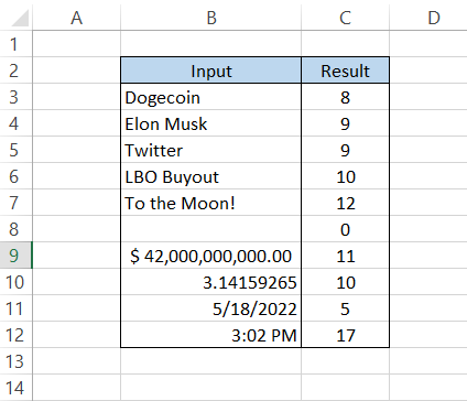
Interpretation

Let's interpret the answers:

• For the text ‘Dogecoin,’ we get the length of the string as 8, which is exactly the number of letters in the text string.
• The text ‘Elon Musk’ has 9 characters in length. There are 8 letters, while the space that separates the first name and last name is another extra character making the total 9.
• We see that the word ‘Twitter‘ only has 7 characters; however, the two additional spaces at the end take the total count to 9.
• Similar scenario, two words separated by a space in ‘LBO Buyout’ takes the length of the string to 10.
• A new case has a special character along with space. Even the special characters will be counted in the result, as evidently seen for ‘To the Moon!’ where the string length is equal to 12.
• When you reference an empty string in the formula, you will get the result as 0.
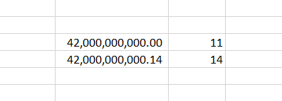
• When you reference numbers, you will get the result of the numerical value we input in Excel. For example, for $42,000,000,000.00, we had input the value to 42000000000 and changed its format to ‘Accounting’ with added dollar symbol. 

When you make superficial changes such as these, it does not increase the length of the string. However, if it had a decimal number, say 42000000000.48, then the length of the string changes to incorporate the decimal and the digits following it, taking our total to 14.

• We have the value of Pi equaling 3.14159265, where the numbers and the decimal point will be calculated for the length of our string.
• Next, we have the date 5/18/2022; as you are aware, dates are stored in serial numbers where 1st Jan 1900 is equal to 1. Since we have referenced a recent date, its serial number is five-digit (44699, to be precise), while if you had referenced the date 1st Jan 1900, the result would be 1.
• Finally, we have the time at 3:02 PM. If you aren’t already aware, you must know that time can also be represented in decimal numbers between 0 to 1, where 0 represents 12 AM, 0.5 represents midday (12. PM), and 0.99999 represents somewhere around 11.59 PM. 

In our case, 3:02 PM can also be represented as 0.626388888888889, which is why the length of our string is equal to 17.

Example 1

The LEN function alone might not have many practical applications, but once you combine it with other compatible functions, it's an upgrade on a whole other level.

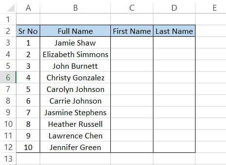
Suppose that you have the employee names in the database as illustrated below:

To find the last name, we will combine RIGHT, LEN, and SEARCH functions. The formula that we will use is =RIGHT(B3,LEN(B3)-SEARCH("",B3)), which will give you the last names in column D as:

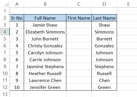
By breaking down the formula, we understand that the LEN function first gives the length of the entire string as a number while the SEARCH function gives another number by pinpointing the position at which the space character is present. 

Finally, the RIGHT function will subtract both the numbers, i.e., RIGHT (10-6) equals 4 characters from the right side, which is 'Shaw' as in cell D3. 

Similarly, B4 has17 characters, while the space character is in the 10th position. So RIGHT(17-10) equals 7 characters from the right, which is 'Simmons' as in cell D4.

Finding the first name doesn't use the LEN function, but the formula used is =LEFT(B3,SEARCH("",B3)), which will give the result as illustrated below:

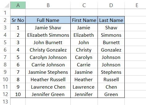
Same logic; however, we use the LEFT function instead of RIGHT and skip the LEN function.

Practical Example 2

If you type a paragraph in a google doc, you can easily count the number of words if you press the key Ctrl + Shift + C, but can you do something similar in Excel? The answer is yes. 

If each word is in a different cell, it is easier, but what if more than 2 words are in the same cell? How would you determine the count of words in that specific cell?

Assume that you have a sentence in Excel as illustrated below:

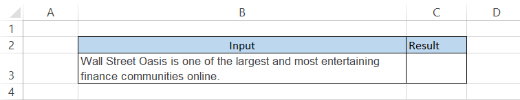
To calculate the number of words in the sentence, we will use the formula =LEN(B3)-LEN(SUBSTITUTE(B3," "," "))+1, which will give us the result as 

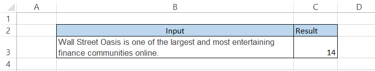
In a nutshell, the number of words is equal to the space characters that separate two different words. Since there is no space in front of the first word, we add 1 to the formula, which gives us the final count of all the words in a sentence.

Practical Example 3

Suppose that you have a text string and need to find the position of a specific word within the sentence. How would you find it? Suppose that the sentence is as illustrated below:

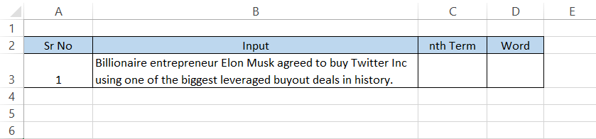
To find the nth term, you will use the combination of TRIM, MID, SUBSTITUTE, LEN, and REPT functions. You might know what the other functions do, but REPT might be relatively new. The function repeats a given character specified 'n' many times.

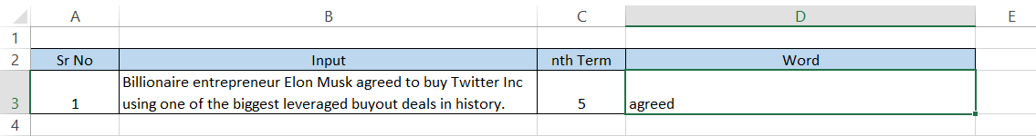
The formula that you will use is =TRIM(MID(SUBSTITUTE(B3," ",REPT(" ",LEN(B3))), (C3-1)*LEN(B3)+1, LEN(B$3))), which will give you the result in cell D3 as:

As you change the nth term in cell C2, the result in cell D2 changes. If the nth term is equal to 5, then the formula will return the result as 'agreed.'

How to use the LEN Function in Excel?

So how does the formula work? Let's break it down into steps:

1. The LEN(B3) finds the sentence's length equal to 121.

2. The use of the REPT function, wherein the Formula REPT("", LEN(B3)) gives us a total of 121 spaces.

3. The formula =SUBSTITUTE(B3," ",REPT("",LEN(B3))) will replace all the single spaces that separate two different words with spaces equal to 121.

4. The result is then enclosed inside the MID function that returns the word based on start_num(the letter from which to return the word) and num_chars(how many letters to return). 

Our  start_num  will be (C3-1)*LEN(B3)+1, where the logic is that each word is separated by 121 spaces, i.e., Billionaire + 121 spaces + entrepreneur, then the start_num directly lands us on our next word. 

The formula so far is MID(SUBSTITUTE(B$3," ",REPT(" ",LEN(B$3))), (C3-1)*LEN(B$3)+1, LEN(B$3)).

5. Even if the word is extracted from the entire string, we don't have to forget the extra spaces that we added in our SUBSTITUTE formula. 

Hence, we use the TRIM function, i.e., =TRIM(MID(SUBSTITUTE(B$3," ",REPT(" ",LEN(B$3))), (C3-1)*LEN(B$3)+1, LEN(B$3))). It removes all the additional spaces from the text, which returns the word based on the nth number you input in cell C3.

Yes, it's a complicated formula and might be difficult to understand. Again, though, breaking it down into various smaller formulas always helps! 

Researched and authored by Akash Bagul | Linkedin

Reviewed and edited by Parul Gupta | LinkedIn

Free Resources

To continue learning and advancing your career, check out these additional helpful WSO resources:

• CHOOSE Function
• CODE Function
• HOUR Function
• HYPERLINK Function
• YIELD Function