TRUE Function

What is the TRUE Function?

A TRUE function in Excel returns the boolean value TRUE. A natural, logical part is often combined with other rational functions such as IF, AND, etc.

Logical functions are the heart of MS Excel. Even though there are many different functions at the users' disposal, the analytic functions take the analysis and number crunching part to another level.

When you input various conditions, you want some of them to return TRUE while other calculations return FALSE. It can be achieved with the help of our function, which helps to produce either the output or the condition as TRUE.

This article will guide you in understanding the Syntax for the function(spoiler alert - the procedure takes in no arguments) and various scenarios in which you can use the process.

Understanding TRUE function

The function is categorized as a logical function that will return the boolean value as TRUE.

When Excel accepts the function as an input, it is the same as the text string 'TRUE.' So, either way, Excel will understand it's the same in conditional statements.

So why do we even have the dedicated function in its name?

The primary reason is to provide compatibility with other spreadsheet programs. Let's say one of your clients prefers using another spreadsheet software instead of Excel. 

If they have a similar logical function used in their reports, then Excel might have thrown some error to you and might be unable to display the result.

To compensate for this, Excel developed the function so that even if the third-party spreadsheet program has the process, it should accurately reflect the same result in MS Excel.

The function was introduced in the Excel 2007 version and has been ever-present in all the subsequent versions.

The Syntax for the function:

=TRUE()

The function does not take in any arguments. All you need to do is begin with the equal sign, followed by the function name and the parenthesis.

You can input the boolean value in three ways:

• As stated above, one is the equal sign, followed by the function name and parenthesis.
• The other begins with an equal sign followed by the function name, and press enter without parenthesis.
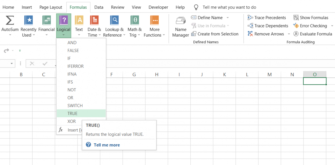
• We can also input the value from the function's library by going into the Formulas tab > Logical drop-down menu > TRUE.

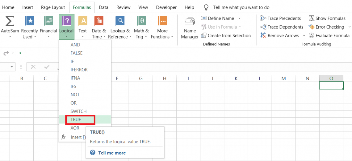
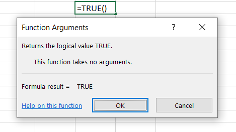
When you click on the function, this will open up the dialog box, after which all you need to do is click on ok.

Examples Of TRUE Function

Here comes the best part -  understanding how the function works. We will see different examples of how you can use the function.

Example #1

Suppose you need to evaluate the number of tests in which Jonathan scored more than 80 marks. The data looks as illustrated below:

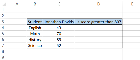
To find the result, we will use the combination of IF and TRUE functions so that the formula is =IF(C4>80, TRUE()), which will give you the result:

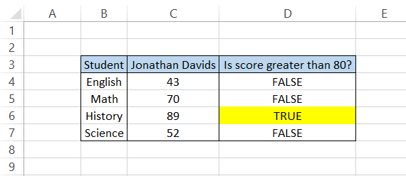
Only in one instance is the score greater than 80 in our data set, as highlighted in cell D6.

Example #2

You might be aware that boolean values are stored in binary format, i.e., TRUE is equal to 1, and FALSE is equal to 0.

We can also use this logic to make calculations in Excel.

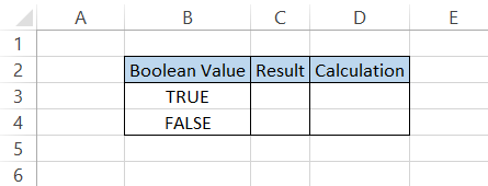
Suppose we multiplied our boolean values by 10, respectively, i.e., =B3*10, which will give us the result, as illustrated below:

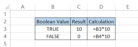
Since TRUE is stored as 1, the result equals the number multiplied when anything is multiplied. As for the FALSE, the result will ultimately be zero since you multiply a number by zero. 

Example #3

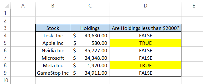
Suppose you work for an institutional investor and need to evaluate all the stock holdings in the portfolio. The portfolio looks as illustrated below:

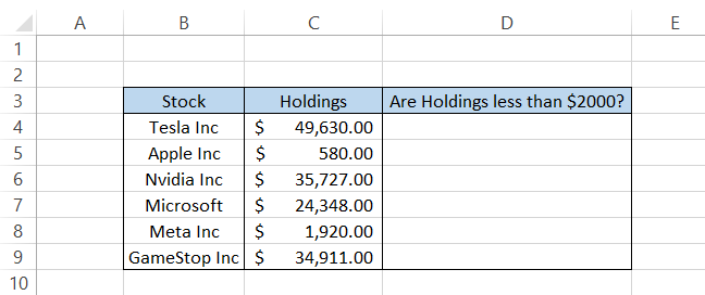
We need to know all the stocks with fewer than $2000. For this, we will use the formula =IF(C4<2000, TRUE()), which will give us the result:

Wait, what if we had thousands of rows of data? In this case, you can input the formula in the conditional formatting tool and let it work its magic.

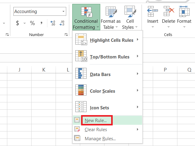
Click on the Conditional Formatting tool from the Home tab > New Rules after selecting the data. 

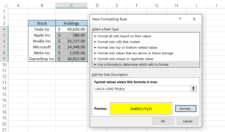
This will open up the dialog box where you input the formula, as illustrated below:

Now, click on OK, and it will highlight all the holdings less than $2,000.

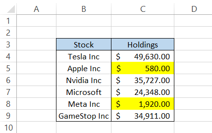
You don't need to add a column and can achieve the same result with the conditional formatting tool.

Example #4

You can also use the combination of AND, IF, and TRUE functions to evaluate multiple conditions.

Suppose that for the dataset below, we want to match the 'Tesla Inc stock purchased for less than $735.

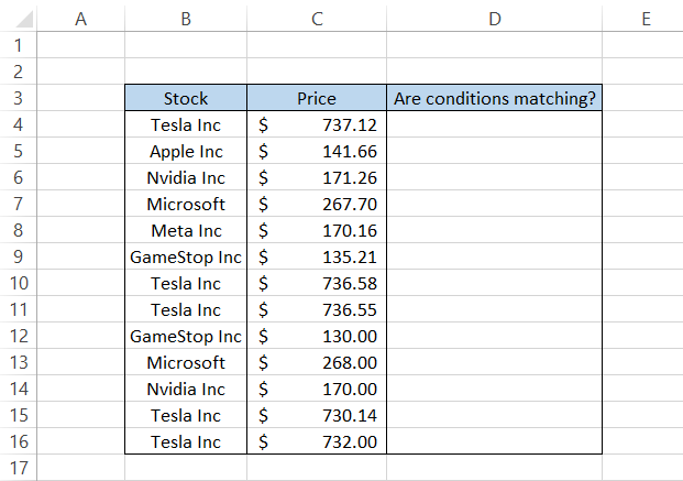
To get the result, we can use the formula, =IF(AND(B4= "Tesla Inc," C4<735), TRUE()), which will give us the result: 

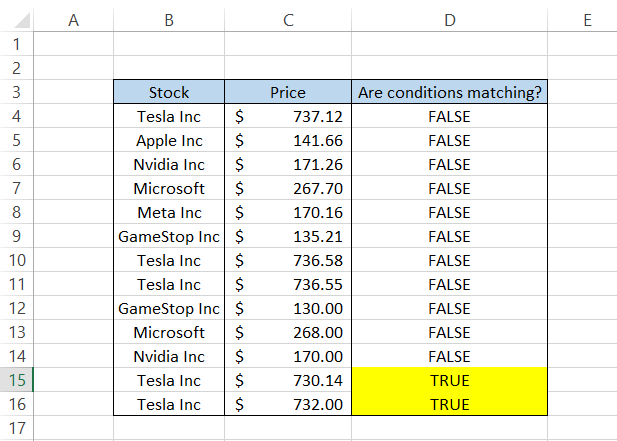
As per the result using the formula, only on two instances, the buying price was less than $735 for Tesla Inc., AND function enables you to input up to 255 additional arguments inside the IF function, thus improving the formula efficiency.

Example #5

Since TRUE is equal to 1 and FALSE is equal to zero, we have different results if we add a combination of them.

Suppose the different combinations are:

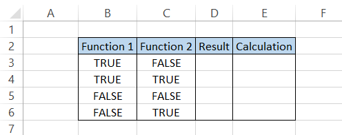
The values input in the cell above is not text strings but the respective functions. So next, we need to perform a simple addition for adjacent cells, which will give you the result:

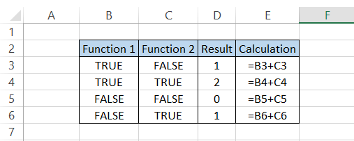
We don't think that the calculations need any explanations. Even though this might be simple, we never know what formula might need this approach!

TRUE vs. FALSE Function

While, on the one hand, TRUE returns the boolean value of TRUE, its counterpart returns the boolean value of FALSE. Both the functions show similarity in having no syntax but return contradictory results. 

While the former stores the value as 1, the FALSE function stores the value as 0.

Again, there are three ways you can use the FALSE function:

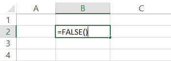
1. You begin with an equal sign, input the function name, and end the formula with the parenthesis.

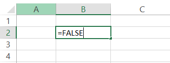
2. The second method is similar to the first, with the only difference being that you don't need to input the parenthesis.

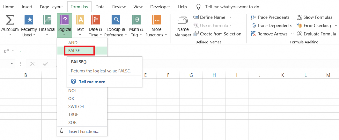
3. Finally, you can also access the function from the library by clicking on the Formulas tab > Logical drop-down box > FALSE.

This will open up the dialog box, as illustrated below:

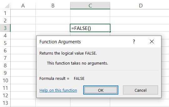
Click on Ok, and you are done.

Suppose that you have the data in Excel as:

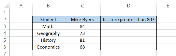
We need to determine what scores are higher than 80 and in which subjects Mike scored less than 80. 

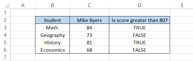
We can use the IF statement, TRUE and FALSE functions for this. The formula will be =IF(C3>80,TRUE(),FALSE()), which will give you the result:

There is an option to use the FALSE with the NOT function. For example, there are two binary numbers - 1 and 0. If you do not have 0 as the binary number, the result would be 1, which equals TRUE. This also works the other way in Excel.

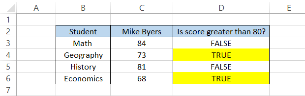
Let's say we use the formula =IF(NOT(C3>80), TRUE()); all the subjects with scores less than 80 will return as TRUE.

Researched and authored by Akash Bagul | LinkedIn

Reviewed and edited by Parul Gupta | LinkedIn

Free Resources

To continue learning and advancing your career, check out these additional helpful WSO resources:

• FV function
• SQRT function
• TRIM function
• XIRR function
• YIELD Function