TRIM Function
An Excel Text Function that removes the additional spaces between words and returns a text string with neither space at the start or end of the text string.


What Is The TRIM Function?
The TRIM function in Excel is an Excel Text Function that removes the additional spaces between words and returns a text string with neither space at the start or end of the text string.
Have you ever worked on Excel files with disorganized data, even in a single cell? For example, we have seen files with street addresses separate cities by hundreds of space characters.
You would ask, wait, what's wrong with that? Isn't it still the correct required value? You can even wholly read it when the cell is highlighted.
The problem arises when you edit the cell to a different value. We must skip all those space characters before replacing the address's cities or street components.
The simple remedy for this problem is to use this function. It removes the spaces, maintains the data integrity, and improves the efficiency of data handling formulas on the same dataset.
In this article, we will see how you can use the function and use it best by incorporating it into your daily Excel activities.
- The TRIM function is an Excel Text Function in Excel is used to remove leading, trailing, and excessive spaces from a text string.
- Users provide a text string as the argument to the TRIM function. The function returns the text string with all leading and trailing spaces removed, and consecutive spaces within the string collapsed into a single space.
- The TRIM function aids in data cleaning and standardization by eliminating extra spaces from text entries, ensuring consistency and accuracy in data analysis and processing.
- The TRIM function can be integrated into formulas and calculations to clean and format text data dynamically, enabling users to automate data cleaning tasks and improve the efficiency of data processing workflows.
Understanding TRIM function
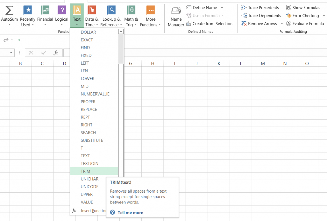
The function is categorized as a text function that removes all spaces between words from the beginning and end of the text string except for a single space between the words.
For example, if you have the text in the spreadsheet as "Apple Inc has more cash than the US Government. "and use the function, the result will be "Apple Inc has more cash than the US Government."
See the magic? The function completely removes all the additional spaces in the sentence. So, even though it has quite a simple purpose, the function is vital in the Excel community.
You must have looked at numerous Excel spreadsheets with many additional spaces, which can be a nuisance when conducting financial analysis.
First and foremost, if you are making an 'apples to apple comparison' for the columns in Excel as a part of the data analysis routine, any cell that contains additional spaces will never return as 'equal' to its counterpart since Excel counts the space as an extra character.
The VLOOKUP and INDEX MATCH can also be affected if the cell contains extra space between the words. As a result, the function forms one of the most essential 'text' functions in the community for all the Excel wizards.
The syntax for the function is:
=TRIM(text)
where,
- text = (required) text string enclosed inside the quotation marks, a cell reference for the text string, or a formula that returns text.
Note
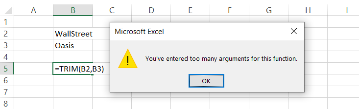
The function only takes in one argument, text, and usually takes in one cell address if referenced in the formula. This means if you try to reference multiple cells in the formula, you will get a dialog box that says, "You've entered too many arguments for this function."

Example Of TRIM Function
Now that we understand the function's syntax let's look at a couple of examples to discuss using it in Excel.
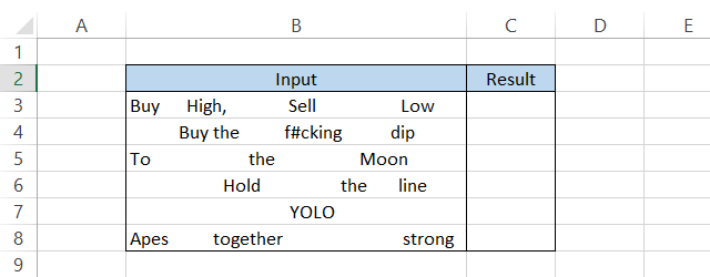
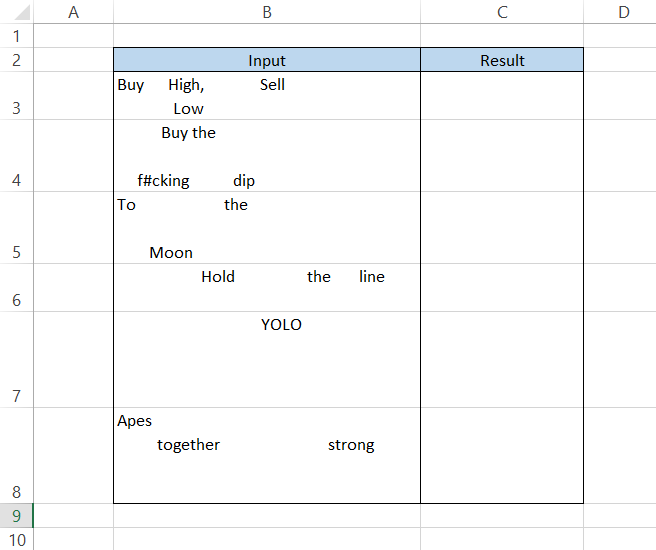
Suppose that you have the data as illustrated below:
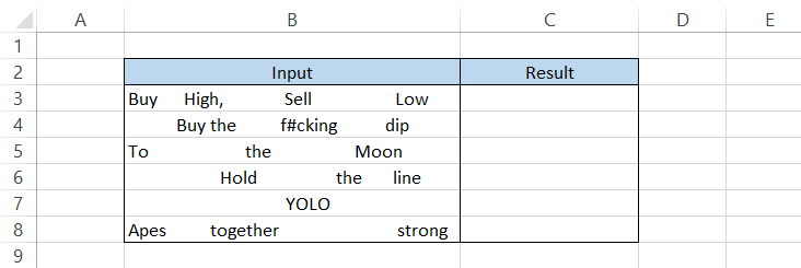
We will write the formula
=TRIM(B3)
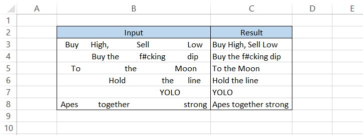
In the cell C3, which will give us the result in the spreadsheet:
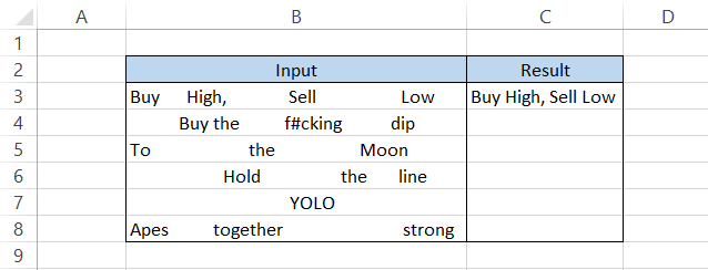
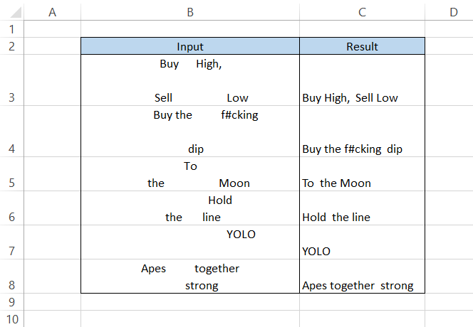
All the spaces between the words were removed immediately using the function, so the space after the word 'low.'
The text string only left one space between the consecutive words and returned the result in cell C3. After dragging down the formula up to cell C8, we will get the result:
The function is designed to remove the space character with a value of 32 in the 7-bit ASCII code system.
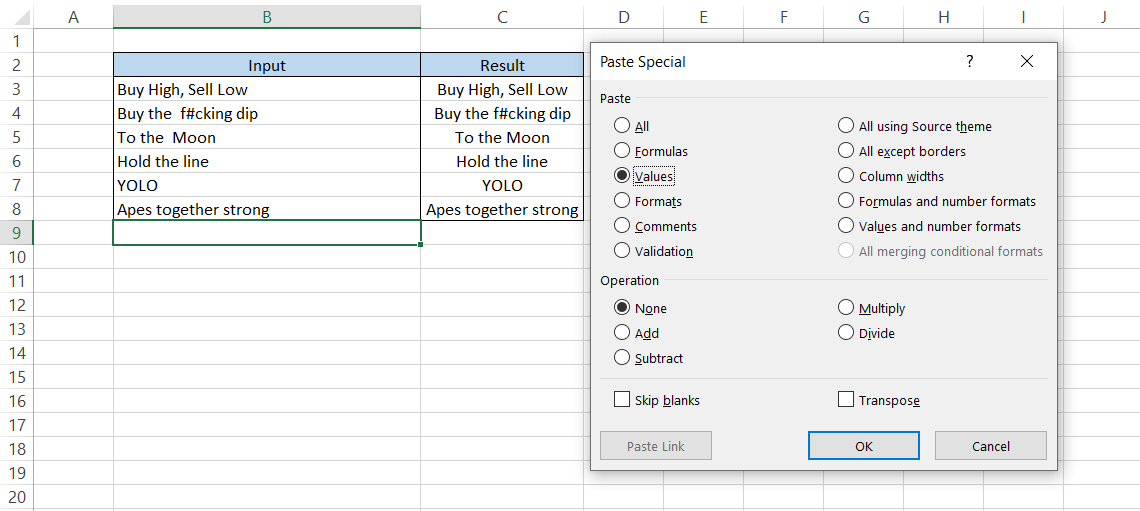
Once the trimmed data is returned, you can PasteSpecial the data into a new cell first by copying the cells using Ctrl + C and then using the keyboard shortcut of Ctrl + Alt + V + V.
This would PasteSpecial the values and avoid any errors in the formula if the data in the B column were to be deleted.
Counting the additional spaces in Excel
There may be instances where you need to determine the number of additional spaces in the text strings. In such cases, we use the LEN function to calculate the length of the enclosed line.
The LEN function also counts the space character in its result, including those that separate two words. So, for example, let's say we have the text strings in Excel as illustrated below:
To count the total number of characters, we will first calculate the length of the text string. Using the formula
=LEN(B3)
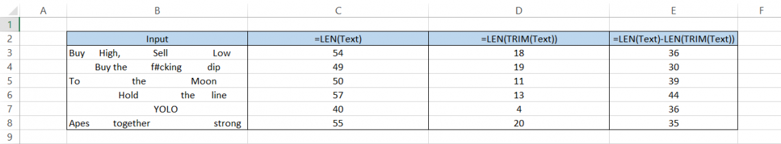
We get the total number of characters in cell B3 as 54. This is because even though there are only 14 letters and 1 punctuation mark, all the extra spaces make up 54 characters.
But this isn't the end of it. Next, we use the function to find the string length without all the extra characters, which returns the result as 18. The calculations behind the total are 14 letters + 1 punctuation + 3 spaces that separate the four words, which equals 18.
Now, if we subtract both the results or use the formula
=LEN(B3)-LEN(TRIM(B3))
it will give the effect of the extra spaces in our cells. The spreadsheet will look as illustrated below:
TRIM Function Illustrations
The function helps to remove all the additional spaces that might be present in a workbook. If you are working on large datasets obtained from third-party resources, there is a high probability you might end up working with this function a lot.
Almost all data cleansing tasks involve this function, which can be used in combination with other parts to provide more accurate and understandable reports.
This section will see practical examples of using the function to obtain clean data.
Practical #1
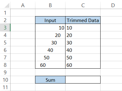
Suppose that, using the VLOOKUP function, you pull in the numerical data in the spreadsheet as illustrated below:
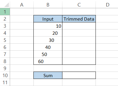
You need to find the sum of the data and remove the additional spaces from the cells. The formula that you will use is =TRIM(B3) which will give you the result as:
Finally, we will calculate the sum of the numbers using the formula
=SUM(C3:C8)
Giving us the result as 0. Wait, what?
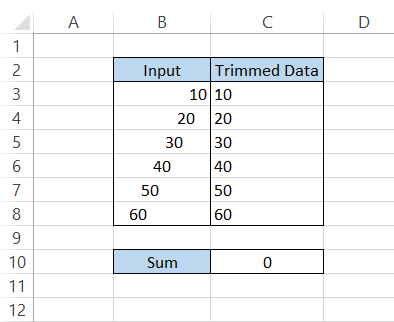
So actually, what happened is that Excel mistook the numbers for text strings and hence could not return the sum for the range of numbers. There are two ways you can overcome this issue in Excel:
Method #1: Multiplying the result with 1
The first method to turn the numbers from their text format into numerical values is multiplying the result from the formulas by 1.
Our formula in the spreadsheet becomes
=TRIM(B3)*1
which will give you the result in the spreadsheet as illustrated below:
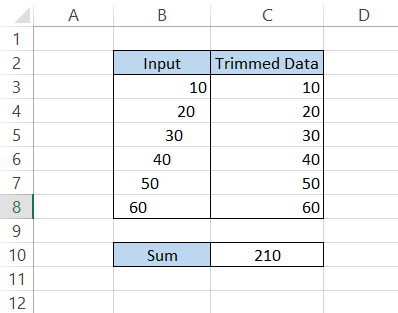
After changing our numbers from 'text format' into their values, we get the sum for the numbers as 210 in Excel.
Method #2: Using the VALUE function
The VALUE function in Excel changes the format numbers represented as text strings into a numerical value.
For example, if you have the date as 1st January 1900 enclosed in the VALUE function, you will get the result as 1(since dates are serial numbers and the first date is Excel begins from 1st January 1900).
The syntax for the VALUE function is:
=VALUE (text)
where,
text = (required) text string inside the quotation marks, a cell reference for the text string, or a formula that returns text
Now, if you combine the VALUE and the function, the latter will remove all the unnecessary spaces between the text. In contrast, the former function will convert the text string into its number format if it holds any numerical values.
The formula becomes
=VALUE(TRIM(B3))
which will give you the result:
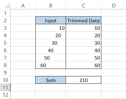
Two methods provide the exact solution; follow what works best for you!
Practical #2
Another function you can use in combination with this function is the CLEAN function. For example, when you download files from the internet or fetch data in CSV format using a database such as Excel, the spreadsheet might import characters that are not printed when the print option is used in Excel.
The function cannot remove such characters solely. Hence, we also need to use the CLEAN function to remove non-printable characters, such as line breaks or text wraps.
Assume that you have the data in the spreadsheet as illustrated below:
As we can see, our data also has line breaks, text wraps, and extra spaces in the cells. Therefore, the formula that we will use in Excel is
=TRIM(CLEAN(B3))
To give you the result in the spreadsheet as illustrated below:
It looks pretty much the same as before.
The formula has worked; all you need to do is PasteSpecial the values in column B, and the spreadsheet line breaks will return to normal.
Copy the result in column C using the keyboard shortcut of Ctrl + C, press Ctrl + Alt + V, and then V to PasteSpecial the values in column B. You will get the result in the spreadsheet as follows:
Practical #3
What if you have two cells with extra spaces but need to combine the value for both in the final results, including removing the areas? For example, assume that you have two input text strings in Excel, as illustrated below:
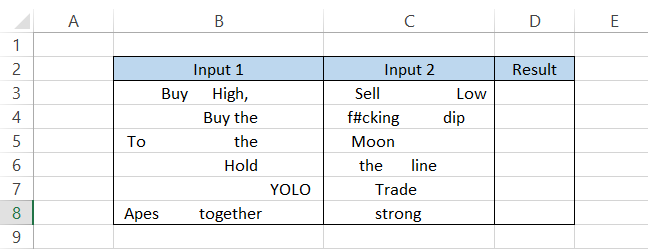
To get the result in a single cell, we will use the formula
=TRIM(B3&C3)
In cell D3, drag the formula down, which will give you the result:
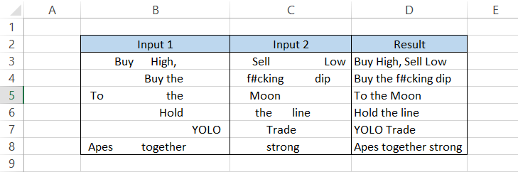
Once you drag down the formula, you will notice that the two input texts concatenate, and all the unnecessary spaces between the text strings are removed, excluding the 'standard' space between two text strings.
This way, you can concatenate numerous text strings together and perform different operations on text strings, such as removing additional spaces using TRIM, returning the text in the proper case using the PROPER function, or even the upper case using the UPPER function.
The magic of concatenation never ceases to amaze us, right

Free Resources
To continue learning and advancing your career, check out these additional helpful WSO resources:


or Want to Sign up with your social account?