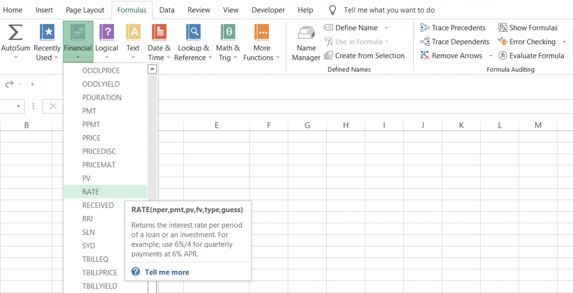
RATE Function
A Financial function in Excel that calculates the interest for a loan or investment over 'n' periods.


What is the RATE Function?
The RATE function is a Financial function in Excel that calculates the interest for a loan or investment over 'n' periods.
If you were in your thirties, you would have imagined buying your own house via a mortgage. However, taking a mortgage from the bank means paying the principal amount plus all the interest payments accrued on the principal over the loan's tenure.
Without interest, a bank would never be able to determine how many additional payments the borrower needs to make to achieve their "American dream" of buying a house.
Why is it important to understand the interest rate? Interest matters because it decides the borrowing cost and the ability of households and firms to spend.
If interests are low, people are more encouraged to buy a car, spend on consumer goods, get a mortgage to buy a house, etc.
On the other hand, a high interest discourages businesses and individuals from spending/investing while encouraging saving.
Ever since the function was added to Excel, it has been an integral part of the workflow of financial analysts and investment bankers.
The function is categorized as a financial function. It calculates the interest for a loan with inputted payments and tenure of 'n' periods.
- The RATE function is used to calculate the interest rate per period for an annuity or investment based on periodic, constant payments and a constant interest rate.
- The function is commonly used in loan and mortgage calculations to determine the interest rate required to amortize a loan or mortgage over a specified period with fixed payments.
- The RATE function can be integrated with other financial functions, such as PV (present value) and FV (future value), to perform more complex financial calculations and analyses.
- RATE function aids in financial planning by helping users determine the interest rate required to achieve specific financial goals or targets, such as saving for retirement or purchasing a home.
Understanding the RATE Function
The RATE function can also be used to determine the required rate on an investment, like equities or bonds, based on the amount invested, the asset's holding period, and the total return.
The function helps easily find periodic interest and monthly interest. It also sees the coupon payments receivable for investments like fixed income or zero coupon bonds in Excel.
The function calculates results using iterations and can have more than one solution in Excel. Microsoft's official documentation for the RATE function states that" if the successive developments of the function do not converge to within 0.0000001 after 20 iterations, the process will return the #NUM! error value".
It means that a loop runs in the background when you use the function, and if the process finds that the loop doesn't return the same value 20 times, then it will return the #NUM! Error.
While this may seem silly, it's one way to avoid a lawsuit. Thomas R. Nicely, in the 1990s, noticed that a bug affected calculations in Pentium systems called the Pentium FDIV bug. The wise have always said, "never make the same mistake twice." "Nicely" done, Microsoft!
RATE function Formula
The syntax for the function is:
=RATE(nper, pmt, pv, [fv], [type], [guess])
where,
- nper - (required) The period (months, quarters, or years) for the interest being calculated.
- pmt - (required) The periodic payments over the loan/investment's life. If pmt is skipped, the pv and fv arguments are needed for the formula.
- pv - (required) pv represents the present value of the loan or investment.
- fv - (optional) fv represents the future value of the loan or investment
- type - (optional) determines whether payments are made at the end of each period (0) or the beginning of each period (1)
- guess - (optional) assumption of what the interest could be. If ignored, the function assumes the rate to be 10%.
The function has been present in all versions of Excel since 2003.
The guess argument only accepts arguments between 0 and 1. For example, if the guess is 15%, then the value you would input in the formula is 0.15

How to use the RATE Function in Excel?
The function has many parameters, so we should go through each individually to better understand the position. Like other formulas, you begin with the equals sign (=) and type the function name in Excel.
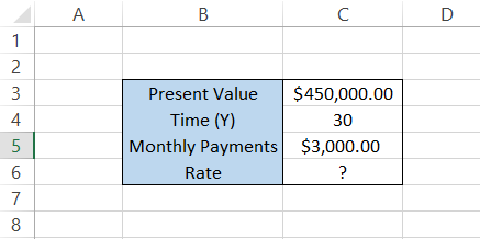
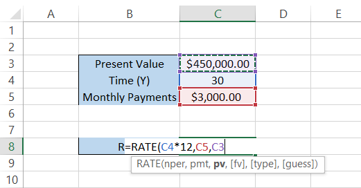
Assume you take out a housing loan of $450,000 for 30 years. To repay it, you need to make $3,000 monthly payments. The data is illustrated below:
Step #1: Time Period (nper)
The first parameter in our formula is the period (nper), which is equal to 30 years in our example. Since we will be making monthly payments for the loan, it is better to represent the period in a similar format as the payments.
So, the formula becomes
=RATE(C4*12, pmt, ,pv,[fv],[type],[guess])
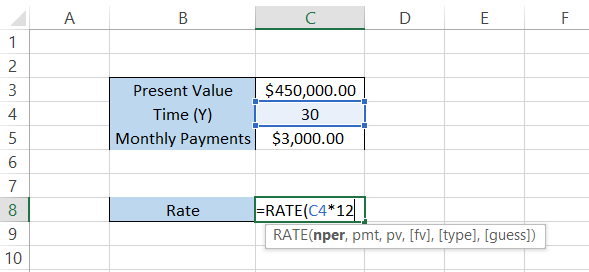
If you intend to make annual loan payments, you do not need to multiply the period by 12.
Step #2: Monthly Payments (pmt)
The following argument in the formula is the monthly payments. We have already adjusted our nper to fit with the data; now all we need to do is reference the correct cell in the formula, which, in this case, is cell C5, i.e., $3,000. Alternatively, you could hard code a payment value into the procedure.
The updated formula in Excel becomes
=RATE(C4*12,-C5,pv,[fv],[type],[guess])
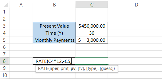
The cash outflows of monthly payments must be represented with a negative sign (-), or else you will get the #NUM! Error.
Step #3: Present Value (PV)
Our present value is the loaned value approved by the bank, which is $450,000. So you know what to do next. Easy peasy, right?
The formula takes the cell reference to the present value,
=RATE(C4*12,C5,C3,[fv],[type],[guess])
These three parameters are more than enough to get the interest for the loan. Use the parentheses to close the formula and press Enter. You will get the interest expressed as a percentage:
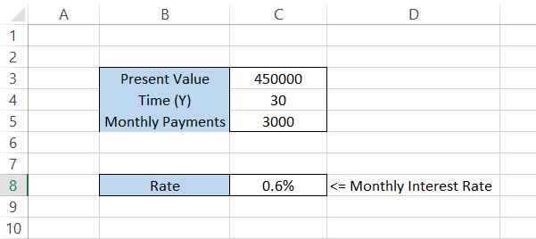
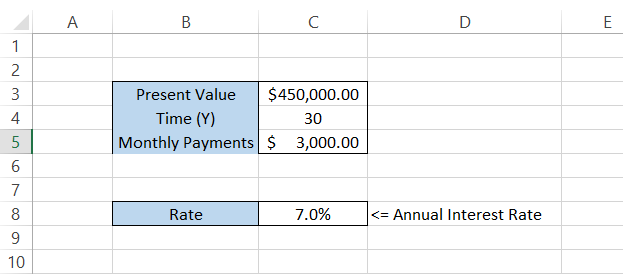
This is our monthly interest on the loan. If you need to find the annual interest, you must multiply the formula by 12, making the formula
=RATE(C4*12,-C5, C3)*12
giving you an interest of 7%.
That's it. Even though there are three additional arguments, using only the "essentials" allows you to find the interest on a loan or the returns on investment.
Step #4: Future Value (fv)
In some scenarios, you won't always have the present value or monthly payments to calculate the interest on the loan or investment.
Assume that one of your friends asks you for a small investment of a million dollars. He says," Bro, I've got a scheme - 25 days and your money will be doubled. I know the person who runs this fantastic crypto project".
You trust him, accumulate the money, and deliver it to him for investment. The data is illustrated below:
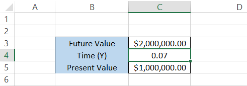
The period of 25 days is represented in decimal form using the formula,
=ROUND(25/365,2)
where 1 is 365 days while 1/365 equals the beginning of the year, i.e., January 1st.
Here, we will use the formula
=RATE(C4,0,-C5, C3)
which will give us the results:
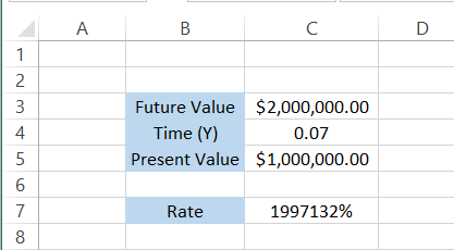
Woah! Those are colossal returns you would only see in movies (yep, you guessed it right!).
Nevertheless, the idea behind this small exercise was to demonstrate that, sometimes, if payments are missing, you can still find the interest based on the future and the present value of the investment or loan.
An important thing to note here is that, since our investment of $1,000,000 was a cash outflow, we either represent it with a negative value in cell C5 or add a minus sign (-) in the formula.
Step #5: Type (1 or 0)
Assume you take out a loan for $100,000 for 5 years and need to make monthly payments of $2000. You have two options: pay at the end of each month (type =0) or at the beginning of each month (type = 1).
The data looks are illustrated below:
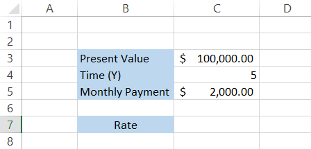
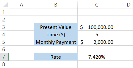
Let's say that you decide to make the monthly payments at the end of each month (default value in Excel). The formula becomes
=RATE(C4*12,-C5, C3,0,0)*12
which will give you the annual interest of 7.42%
However, if you make payments at the beginning of each month, the formula becomes
=RATE(C4*12,-C5, C3,0,1)*12
which will give you the result in the spreadsheet as 7.69%.
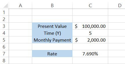
The difference between interest rates, though minor, is quite evident. Therefore, anyone who would opt for the loan will choose the first option since it offers a lower interest rate.
Step #6: Guess
The guessing parameter is rarely ever used by financial analysts. This is because the logic behind the guess value is that it helps the function converge on the result faster if the 'guess' value is similar to the actual value.
The default value Excel uses to guess the interest is 10%.
You can skip this argument or take an educated guess as to what the interest would be. No matter what, it definitely won't affect the result. For example, we will guess the interest will be 70%.
The formula becomes
=RATE(C4*12,-C5, C3,0,1,70%)*12
which still gives you the result in Excel as 7.69%:

RATE Function Examples
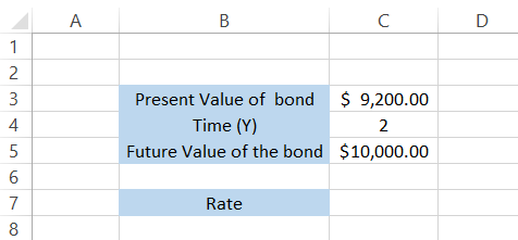
Assume that you purchase zero coupon bonds worth $9,200 with a face value of $92 and a holding period of 2 years. What would be the rate of return on the bonds at the end of the investment period?
Since the zero coupon bonds yield the total face value at the time of maturity, i.e., $100, the future value of the bonds is equal to $10,000. The data is illustrated below:
The formula that we will use to calculate the coupon is
=RATE(C4,0,-C3, C5)
which will give you the result of 4.257%.
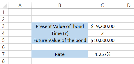
In summary, the return on the zero coupon bond is equal to 4.257% for the two-year holding period when the bond's future value is $10,000 and the present value is $9,200.
Zero coupon bonds don't make any coupon payments to their investors. Instead, they are usually issued at a discount price and redeemed at the par price. This makes up for the coupon payments in the form of 'phantom interest' that accrues yearly.
Let's look at another example to drive home our understanding.
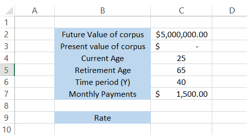
Assume that you are looking to build a retirement account and plan to diversify your investment portfolio in different avenues. You're currently 25 years old and want to retire when you're 65.
Currently, you have $0 to support your retirement, but you are willing to invest $1,500 monthly.
You decide that a retirement account of $5 million would be enough to fulfill your needs for 20 years after age 65. The data in Excel is illustrated below:
To calculate the required rate to reach the retirement account value of $5 million, we will use the formula
=RATE(C6*12,-C7, C3,C2)
and multiply it by 12 to get an annualized return of 7.840%.
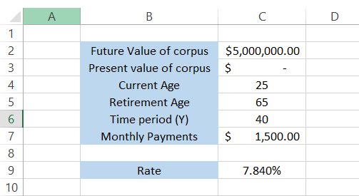
To achieve your retirement goal, you need to diversify your portfolio so that it yields a compounding annual interest of 7.840%.
Last we heard, WSO Alpha was making a whopping 17% annualized returns on its diversified portfolios.

Free Resources
To continue learning and advancing your career, check out these additional helpful WSO resources:


or Want to Sign up with your social account?