MAX Function

What is the MAX Function?

MAX Function in Excel is categorized as a statistical function that returns the maximum value from numerical values, cell references with numerical values, or the range of cells with numbers. 

Recently the team was working on reconciling the WSO Alpha tradebook. We decided to assess how good analytical skills the intern had. The objective was to find the maximum percentage of profits, latest settlement dates, and largest profit share from various accounts at WSO Alpha. 

He said," Alright, give me ten minutes or so, and I will deliver the file back." And boy, he did stand up to the challenge.

Using the combination of INDEX-MATCH and the MAX function, he could return the latest settlement date by comparing it to the other dates in the file and the profit metrics. 

It shows just how progressive GenX learning competence has been. Ten years ago, we would struggle with the essential Excel functions, let alone work on the complicated nested formulas.

Assuming that you might have read about using the INDEX-MATCH function, this article will otherwise focus on how to use the MAX function to improve financial reporting and analysis in Excel.

For example, if you have three numbers, 18, 36, and 21, the MAX function will give the result 36. 

Not just numbers, if you have three or more dates, such as 14th March 2022, 18th March 2022, and 10th March 2022, the result that Excel will return will be 18th March 2022.

MAX function will ignore text values, boolean values such as TRUE and FALSE, and empty cells in its result.

MAX function Formula

The syntax for the function is:

=MAX(number1, [number2])

where,

• number1 = (required) first numerical value or the referenced range of cells consisting of numerical values.
• number2 = (optional) second numerical value or the referenced range of cells consisting of numerical values.

You can use up to 255 additional arguments in the function, i.e. (number1, number2,....number256), that are numerical values or a referenced range of cells.

You can use the function in two ways - either from the function's library or as a worksheet formula.

a. From the function's library

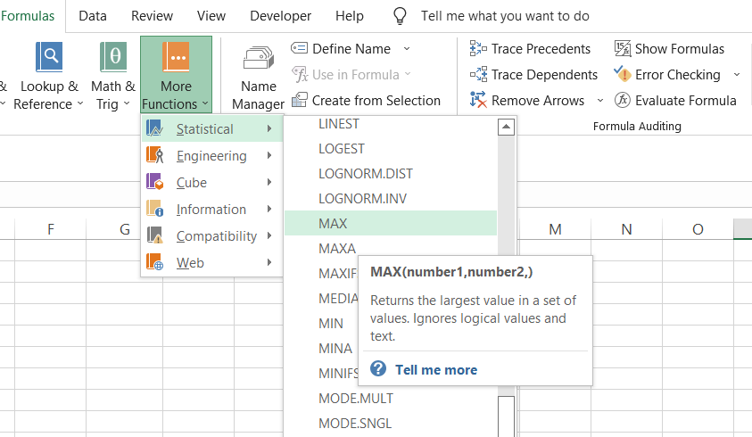
To use the function from the library, select the cell in which you require the result > click on the Formulas tab > More Functions > Statistical, and then select the MAX function.

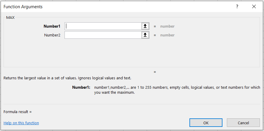
It will open up the argument dialog box where you add all the inputs per the function's syntax and click on Ok to get the result in the selected cell.

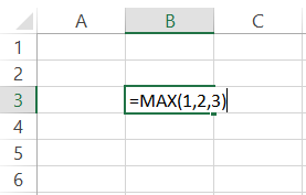
b. As a worksheet formula

The easiest and most efficient method is using the function as a worksheet formula.

You begin with an equal sign(=), type in the function name, and finally input the arguments inside the parentheses, which returns the final result in the selected cell.

How to use the MAX Function in Excel?

The function is pretty straightforward. It does what you ask for - give the maximum input values. We will see a couple of examples to help you understand the function better.

Example 1

Assume we have the trade book data as illustrated below. We must find the most significant transaction value for the last 20 days. 

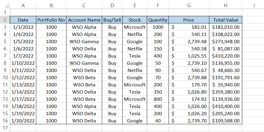
For this, you will use the formula =MAX(H3:H16), which will run a detailed scan through column H for the most considerable transaction value and return the result as $410,400.00. Piece of cake, right?

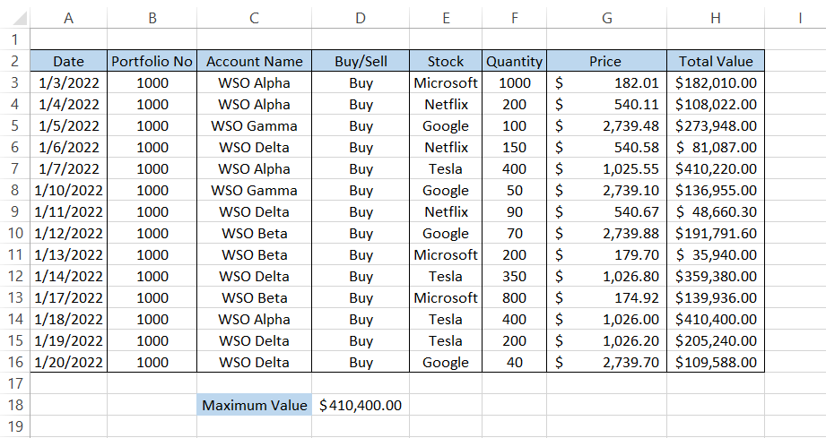
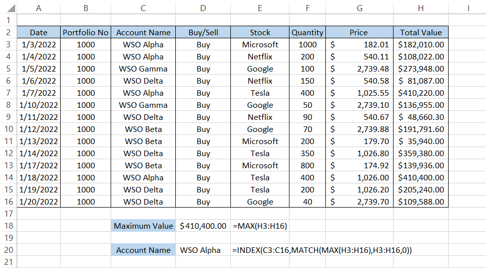
Let's take it a step further. Let's return the 'Account Name' based on the maximum transaction value. 

If you don't know what the maximum value is from the range of cells and you need to return a corresponding cell value, the formula that you need to use is =INDEX(C3:C16, MATCH(MAX(H3:H16), H3:H16,0)) which will give you the result as:

Example 2

Don't we all love the examples based on the student's examination scores? 

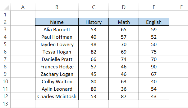
Assume that as a teacher, you must find the most marks scored by the students in the classroom of ten. 

The student's scores in History, Math, and English subjects are as illustrated below:

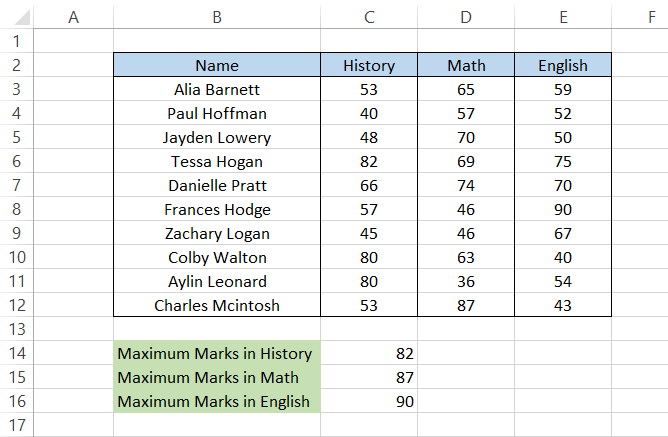
If you need to find the maximum marks scored in a History subject, you will use the formula =MAX(C3:C12) to give you the result of 82. 

On a closer look, you will find the result is correct, and the name of the student who scored the highest in History is Tessa Hogan. To find the most marks scored in Math and English, the only change you will see in the formula is the referenced range of cells. 

The formulas will become =MAX(D3:D12) and =MAX(E3:E12) for Math and English, respectively, to give you the result:

 MAX and other functions

Some functions in Excel go well with others and take the data analysis a step further. MAX function is no exception as well. 

In this section, we will see different instances where you can use the MAX function to improve efficiency while working on a large data set.

a. MAX and IF

Excel 2016 and below users, we hear you. The SUMIF function returns the sum of the numerical values that meet specified criteria, while the COUNTIF function lets you count the values based on the input condition. 

But how do we find the MAX value based on specific criteria? 

As you might already know, a specific function does not exist that will let you find the MAX based on the input criteria. In such a case, you can use the combination of MAX and IF functions to return the required result in Excel. 

Assume that you are a day trader and have undertaken trades as illustrated below:

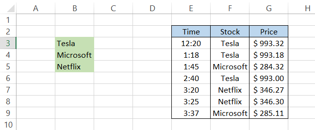
It would be best to find the maximum price you paid for each stock for the day. All the supplies in the trade book are recurring values since you have only traded in three securities - Tesla, Microsoft, and Netflix. 

To check the maximum price for each stock, you will use the formula =MAX(IF(B3=$F$3:$F$9,$G$3:$G$9)) in cell C3, which will give you the result of $993.32. 

After dragging down the formula, you will get the result:

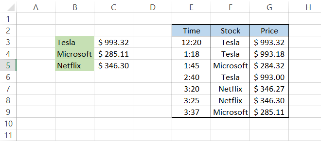
The maximum price you paid for Tesla was $993.32, Microsoft was $285.11, and Netflix was $346.3.

 b. MAX and nested IF

When you need to find a maximum value based on multiple conditions, you can use the combination of nested IF and MAX functions.

Assume that you have the stock trading data as illustrated below:

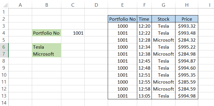
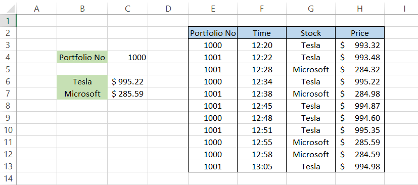
You need to find the maximum price you paid for both Tesla and Microsoft stock in 'Portfolio No' 1001. 

To get the result, you will use the formula =MAX(IF(B6=$G$3:$G$13, IF($C$4=$E$3:$E$13,$H$3:$H$13))) to give you the effect as 

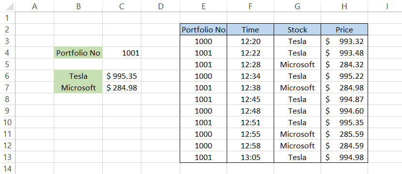
The maximum price you paid for Tesla in portfolio 1001 is $995.35, while for Microsoft, you paid $284.98. If you change the portfolio number to 1000, the result will be as illustrated below:

As you can see, Tesla was purchased for $0.13 lower in portfolio number 1001 than in portfolio number 1000, while the Microsoft stock was purchased at a premium price in portfolio 1000 which cost an additional 0.61$ per share.

The only question that remains is - how does the formula work? Let's break it down to analyze:

1. Using the first IF function, we evaluate all the portfolio numbers equal to 1001 in ranges E3:E13. Since we use an array formula, we get a TRUE or a FALSE if the match is found.

2. The resultant array for the first condition would be {False, True, True, False, True, True, False, True, False, False, True}

3. Another IF condition evaluates to find 'Tesla' in range G3:G13, which gives the resultant array as {True, True, False, True, False, True, True, True, False, False, True}

4. When you combine both these arrays, we will get the resultant array as {False, True, False, False, False, True, False, True, False, False, True}

5. Based on this resultant array, we find only the values $993.48, $994.87, $995.35, and $994.98.

6. Finally, the MAX function finds the maximum value out of these four values equal to $995.35.

The conditional arrays mentioned above are for condition 'Tesla' and would change for state 'Microsoft.' 

 MAXIFS function

If you don't prefer using nested IFs to input multiple conditions, you can use the MAXIFS function in Excel. The downside to using the MAXIFS is that it is only available to Excel 2019 and Excel 365 users. 

If you don't use either, you might have to use the MAX and IFS function combination to run a multiple criteria evaluation to find the maximum value.

The syntax for the MAXIFS function is:

=MAXIFS(max_range, criteria_range1,criteria1,[criteria_range2,criteria2]

Where,

• max_range = (required) the range from which you need to find the maximum numerical value 
• criteria_range1 = (critical) range of cells which will be evaluated by criteria1
• criteria1 = (required) the expression that evaluates the criteria_range1 to find the maximum value
• criteria_range2 = (optional) range of cells which criteria2 will evaluate
• criteria2 = (optional) the expression that evaluates the criteria_range2 to find the maximum value.

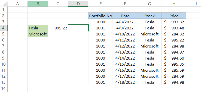
Returning to our example from the previous section, let's say you need to find the maximum price you paid for Tesla stock in portfolio 1000.

The formula that you will use is =MAXIFS(H3:H13, G3:G13, "Tesla," E3:E13, "1000") which will give you the result as 

Similarly, suppose you need to find the maximum price paid for Microsoft in portfolio 1001. In that case, you will alter the formula to =MAXIFS(H3:H13, G3:G13, "Microsoft," E3:E13, "1001") to give you the result in cell C5 as illustrated below:

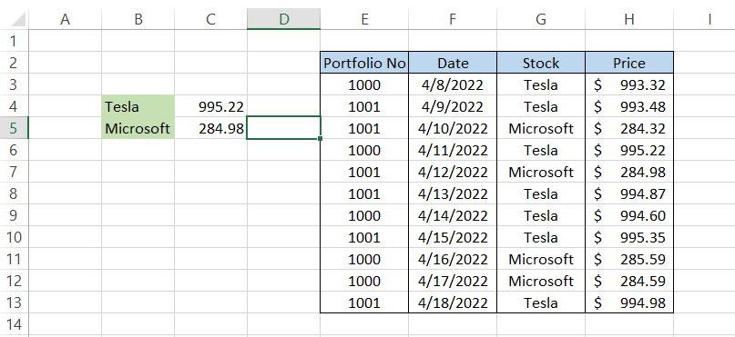
To avoid constantly changing the formulas, you can reference the 'Portfolio No.' and 'Stock' values.

MAX and Conditional Formatting

Conditional Formatting in Excel is so damn underrated. You can run any criteria through conditional formatting by setting up the 'rules' and highlighting the cells that match the specified criteria.

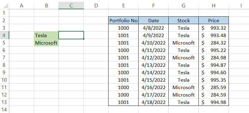
Assume you have the trading data as illustrated below: 

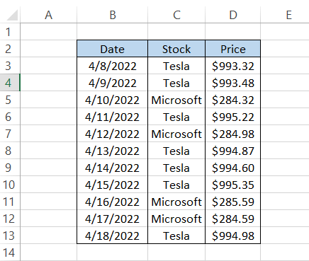
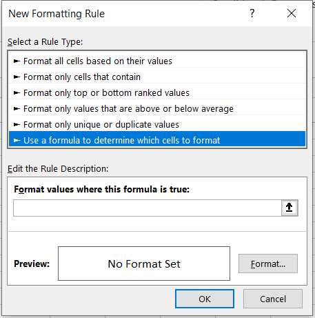
Suppose that you need to highlight the latest date in your spreadsheet data. First, select the range of cells B3:B13 and then from the Home tab, click on Conditional Formatting or use the keyboard shortcut of Alt + H + L + N to set up a new Formatting Rule in the dialog box as:

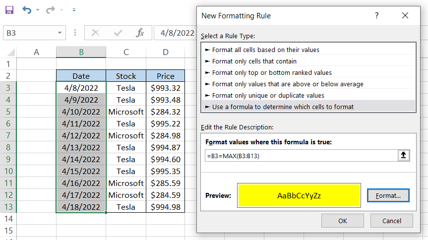
Here, we will set up the MAX formula as =B3=MAX(B3:B13) as we want Excel to know our beginning value first. Excel would highlight all the cells in the specified range if you had just used the formula as =MAX(B3:B13). 

Next, we select the background color for the cell that accepts the criteria.

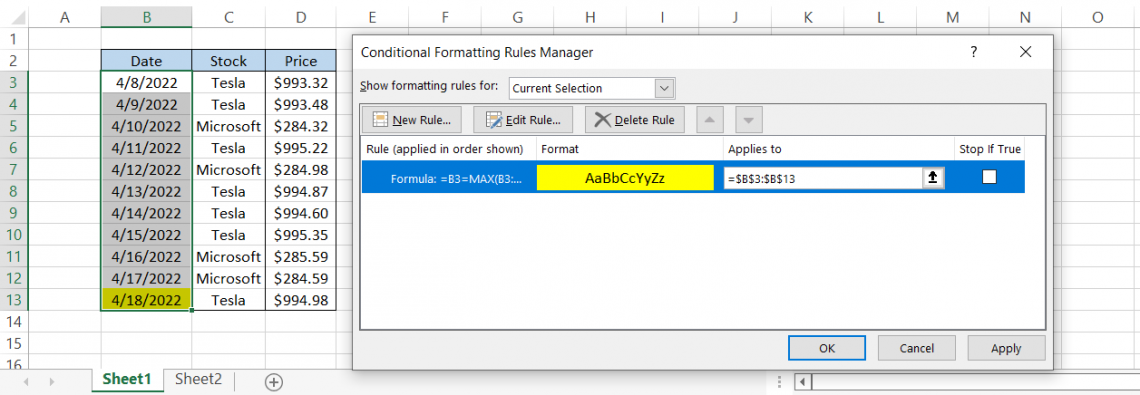
When you click on Ok, the latest date in the spreadsheet, i.e., 4/18/2022, will get highlighted. You can additionally check the rule that you input in Conditional Formatting by using the keyboard shortcut Alt + H + L + R.

Free Resources

To continue learning and advancing your career, check out these additional helpful WSO resources:

• CODE Function
• MINIFS Function
• PRICE Function
• RATE Function
• SUM Function