MIN Function
An Excel Statistical Function that is utilized to find the smallest number in the given data set.


What is the MIN Function?
The MIN Function is an Excel Statistical Function that is utilized to find the smallest number in the given data set.
The MIN Function calculates the minimum number in the data set, ignoring the text, ignoring empty cells, and logical values like TRUE and FALSE.
The function can be useful when determining the lowest expense, score, minimum salary, pay, or even the minimum time taken to complete the task.
When someone visits a supermarket, they always look for a good product discount. If two companies, A and B, manufacture bread, and the packet costs $4 and $4.45, the person would obviously opt for the former product.
The rationale behind a person's action might differ, but the point we want to make is that the person looks at both products' prices and opts for the lower-priced option.
The MIN function uses a similar approach: It scans a set of numerical values and ultimately returns the number that is the minimum for the entire group.
If you are working on numbers in Excel, looking at one or two numerical values is relatively easy. But what if you had thousands of rows of data? It would take days to evaluate all those numbers and find the minimum value among them.
In this article, we will examine the function's syntax, how the process works, and some examples to better understand the position.
- The MIN function will return the minimum value from a set of numerical values or a range of cells consisting of those numerical values.
- The MIN function calculates the minimum value among a set of numbers. It is commonly used in data analysis, financial modeling, and various other applications to identify the smallest value in a dataset.
- The MIN function can handle numeric values, including integers, decimals, and fractions. It can also handle date and time values, where earlier dates or times are considered smaller than later ones.
- Besides the #VALUE! error mentioned earlier, the MIN function may also return a #NUM! error if any of the specified arguments are invalid or if the result exceeds the numerical limits of Excel.
Understanding the MIN function
The MIN function is categorized as a statistical function that returns the minimum value from numerical values, cell references with numerical values, or the range of cells with numbers.

For example, if you have three numbers, 18, 24, and 48, the MIN function will return the result as 18.
You might be aware that dates are stored as serial numbers in Excel. For example, the starting date in Excel is 1st January 1900, which is held as serial number 1.
When you compare two dates for minimum value, say, 6th July 2022(serial number is 44748) and 4th April 2022(serial number is 44655), then Excel will return the minimum value, which is 4th April 2022.
Even the time, stored as decimal numbers in Excel, responds to the function returning the most negligible value. So, for example, if you have the time as 11:30 AM, 1:00 PM, and 4:35 PM, then the function will return the result as 11:30 AM or the decimal number corresponding to the time.
MIN function will ignore the boolean values such as TRUE or FALSE, text values, and empty cells in its result.
MIN Function Formula
The syntax for the function is:
=MIN(number1,[number2])
Where,
- number1 = (required) numerical value or the referenced range of cells consisting of numerical values
- number2 = (optional) second numerical value or the referenced range of cells consisting of numerical values
You can input up to 255 additional arguments in the function, i.e., (number1,[number2],[number3]....[number256]), that are numerical values or a referenced range of cell.
How to Use the MIN Function in Excel
There are two ways you can use the MIN function in Excel - from the function's library or as a worksheet formula.
Method 1: From the functions library
Functions are the predetermined formulas where you need to input the argument, and Excel takes care of the rest of the business. To use the MIN function, please follow the steps below:
- First, select the cell in which you intend to return the result.
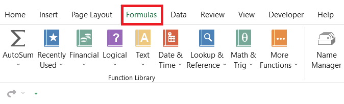
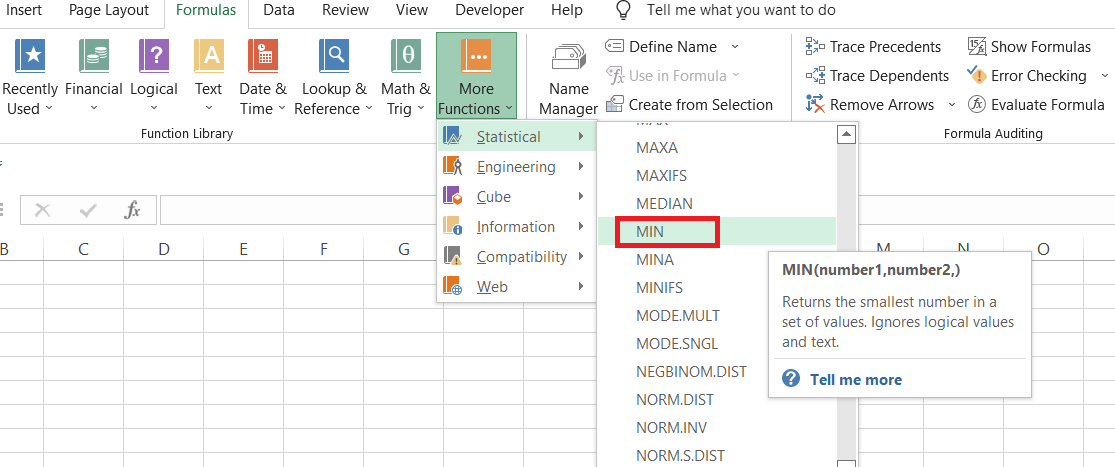
- Click on the Formulas tab > More functions > Statistical, and select the MIN function.
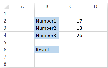
- This will open up the dialog box, as illustrated below:
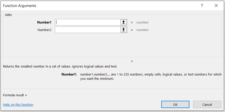
- Here you input the arguments, i.e., the numbers you need to compare to find the minimum value. For example, we will input the Number1 as 13 and Number2 as 7, as illustrated below:
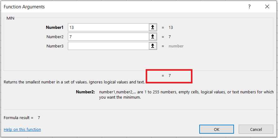
- As you can see, the function already previews the minimum value from the two arguments.
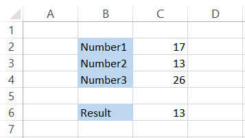
- Finally, click ok, and you should get the result as 7 in the selected cell.
Method 2: As a Worksheet formula
Another way that you can use the functions is via a worksheet formula. Most analysts prefer to use this method since it saves a lot of time by not going through the function library and searching for the desired function, plus it gives greater flexibility.
But forget not! They are Excel wizards who have been working on spreadsheets for ages. If you are a beginner, we urge you to explore different functions in the library and then take the challenge head-on with the formula.
Suppose that you have the data in Excel, as illustrated below:
All we need to do is begin with an equal sign in cell C6, type in the function name and then reference the cells as arguments. The formula will be =MIN(C2, C3, C4), which should give you the result:
You might think we can only reference 256 numbers in the formula, right? We have got a two-letter word for you - 'No.' You could get the same result using the formula as =MIN(C2:C4).

This means you can reference a range of cells as a single argument. For example, if a field consists of thousands of rows and columns, you can input 255 other contents, which Excel would evaluate and return the minimum value.
This also opens up the possibility of comparing numerical values on different worksheets( 255 spreadsheets, to be precise + 1 spreadsheet, which would be used for the formula)
So you can probably imagine how enormous the function's scope can be if you play around with the range you input as an argument to find the minimum value.

MIN Function Examples
Here comes the best part of the articles - some examples that would help the function to get deep-rooted in your mind.
Example 1
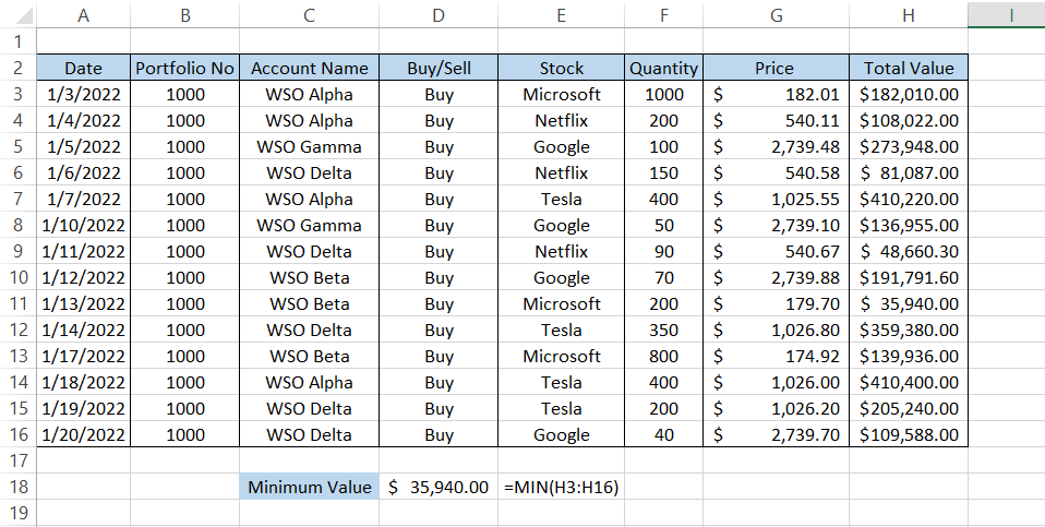
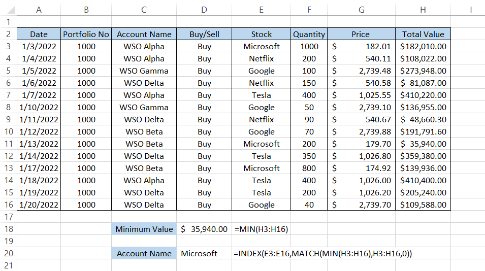
Assume that you have the trade book data as illustrated below. Next, we need to find the minimum transaction value for the last 20 days.
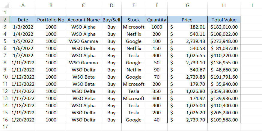
Here, we will use the formula =MAX(H3:H16), which will evaluate all the numerical values in the defined range for the minor matter, i.e., $35,940.
We know that using the VLOOKUP function allows us to get the values of the corresponding cells in the duplicate rows. This way, we can probably find the 'Account Name' or the 'Stock' using the nested formula for the minimum value.
But wait! Did you forget VLOOKUP does not support left lookups? In that case, our only other options are XLOOKUP or the INDEX MATCH. Unfortunately, most Excel users don't have the former function since the Excel 365 version only supports it.
To find the corresponding cell value to our minimum function result, we can use the formula =INDEX(C3:C16, MATCH(MIN(H3:H16), H3:H16,0)), to get the 'Account Name' as:

Similarly, if you need to find what Stock was bought for the minimum amount of $35,940, the only change the formula would see is the range in that range would change to E3:E16 from C3:C16.
The formula would be =INDEX(E3:E16, MATCH(MIN(H3:H16), H3:H16,0)), to give you the result as Microsoft.
Example 2
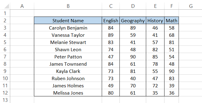
Suppose you need to evaluate the student test scores for different subjects. The data looks as illustrated below:
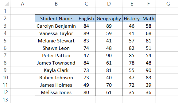
To find the minimum score on the English test, we will use the formula =MIN(C3:C12), which will give us a result of 47.
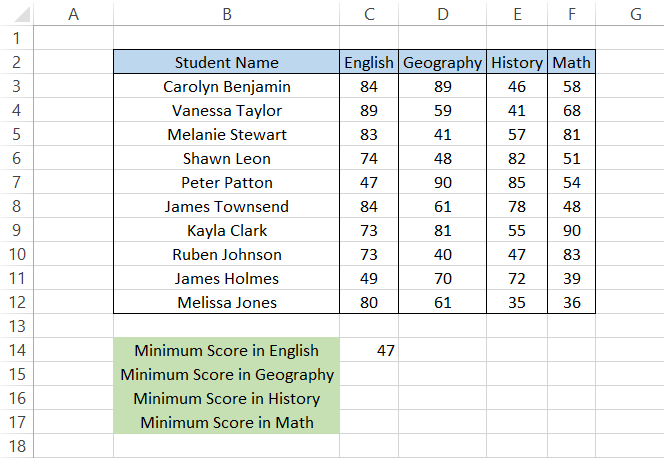
On closer inspection, we can find that those test scores belong to Peter Patton. Using the INDEX MATCH formula, you can also find the 'Student Name.'
Similarly, we will reference the ranges to find the minimum scores in the rest of the subjects
as:
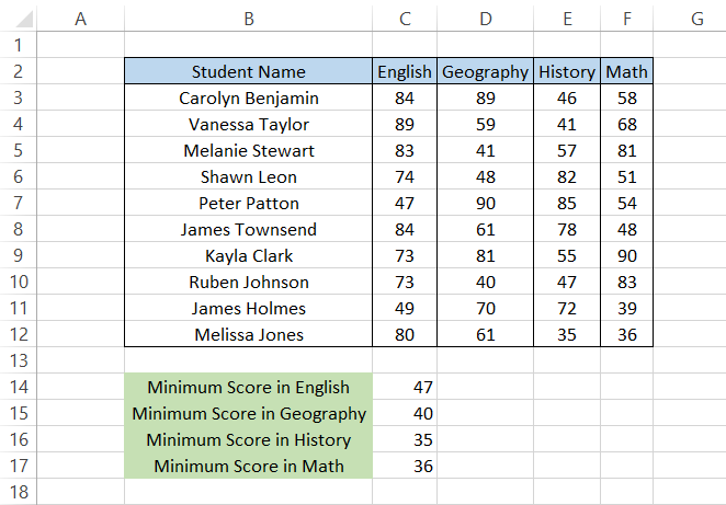
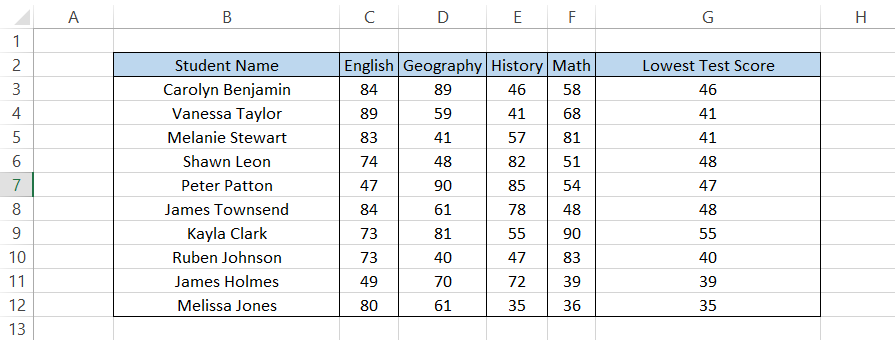
The minimum test scores in Geography, History, and Math are 40, 35, and 36, respectively.
MIN and Other Functions
Everyone in the Excel community would agree that MIN is quite a versatile function. It goes well with IF, AND, OR parts, etc.
MIN along with the IF function
Assume you have the test scores for the students, as illustrated below:
Suppose you need to evaluate what was the lowest score for Carolyn Benjamin in all the examinations.
Here, we will use the formula =MIN(IF(B3=$B$3:$B$12, C3:F3)) in cell C3, which will give us the result as illustrated below:
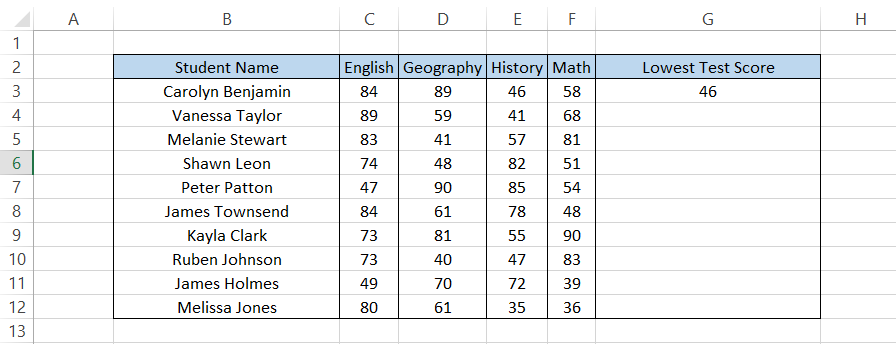
Out of English, Geography, History, and Math, Carolyn Benjamin scored the lowest in History, i.e., 46.
By dragging down the formula, we can get the result for the rest of the cells as follows:
We have the COUNTIF and the SUMIF function in Excel to count or sum values based on a single criterion. What we lacked was finding a minimum value based on single criteria.
This can be overcome with the help of the combination of MIN along with IF functions.
Since this is an array formula, you must press Ctrl + Shift + Enter to get the result.
MIN along with nested IF
You can use the nested IF functions to evaluate a minimum value based on multiple conditions.
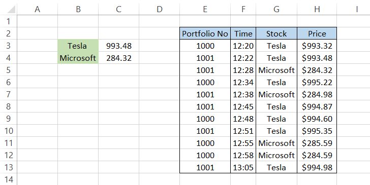
Suppose that you have the trading data, as illustrated below:
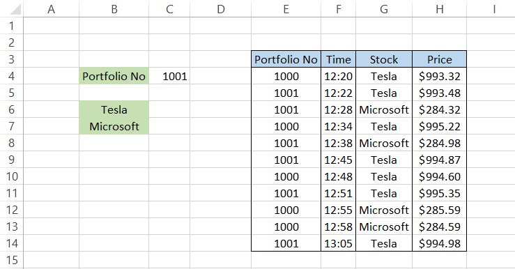
Next, we need to find the minimum price paid for Tesla in Portfolio No 1001. Here, we will use the formula =MIN(IF(C4=$E$4:$E$14, IF(B6=$G$4:$G$14,$H$4:$H$14))), which gives us the result:
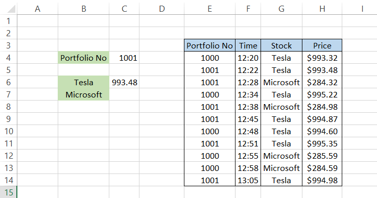
First and foremost, we need to understand that this is an array formula, i.e., you need to press Ctrl + Shift + Enter after you input the formula.
So, how does the formula work? First, let's break down the procedure into two steps:
- The first IF function in the formula evaluates to find all the 1001 portfolio numbers in the range E4:E14. The array returns the result as {False,True,True,False,True,True,False,True,False,False,True}.
- We nest in another IF condition to find 'Tesla' in range G4:G14. This time, when the match is found, the array returned is {True,True,False,True,False,True,True,True,False,False,True}.
- When you combine these array results, we only need the' TRUE' result in both arrays. The final resultant array would be [False,True,False,False,False,True,False,True,False,False,True}.
- As you can see, four values match our IF conditions, which are $993.48, $994.87, $995.35, and $994.98.
- Finally, the MIN function waves its magic wand to find the minimum value from 'those' four prices, which is equal to $993.48
Drag the formula down and get the minimum price for Microsoft using the conditions.
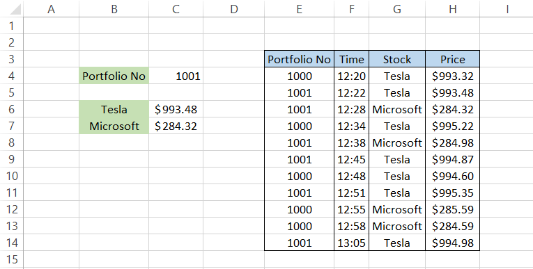
Once you input the formula, you can quickly check the minimum values for Tesla and Microsoft by changing the portfolio number in cell C4.
Since this is an array formula, you must press Ctrl + Shift + Enter to get the result
MINIFS function
If you feel that nested IFs are a bit complicated, you can use the MINIFS function that takes in multiple conditions to find the minimum value. However, the drawback to the process is that it is only available to Excel 2019 and Excel 365 users.
If you have an earlier version, we advise you to stick to nested IF formulas to input multiple conditions for finding the minimum value.
The syntax for the MINIFS function is:
=MINIFS(min_range,criteria_range1,criteria1,[criteria_range2,criteria2])
where,
- min_range = (required) The range from which you need to find the minimum value
- criteria_range1 = (required) range of cells, which will be evaluated by criteria1
- criteria1 = (required) the expression for evaluating the criteria_range1 to find the minimum value
- criteria_range2 = (optional) range of cells, which criteria2 will evaluate
- criteria2 = (optional) the expression for evaluating the criteria_range2 to find the minimum value
You can input up to 126 range/criteria pairs in the formula to test multiple conditions and ranges.
Suppose we want to find the minimum price paid for Tesla stock in portfolio 1001. The data looks, as illustrated below:
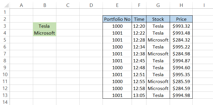
Here, our two different criteria are:
- Tesla
- 1001
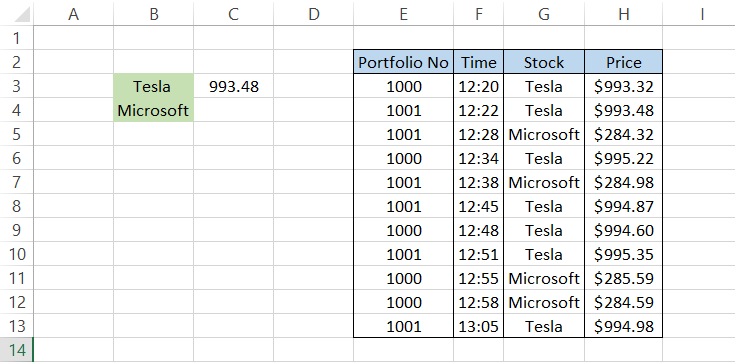
By incorporating them into our arguments, we will be using the formula as =MINIFS(H3:H13, G3:G13, "Tesla", E3:E13, "1001"), which should give us the result:
Similarly, to find the minimum value for Microsoft in portfolio no 1001, the formula will be =MINIFS(H3:H13, G3:G13, "Microsoft", E3:E13, "1001"), which should give us the result:
This way, you can input 126 criteria/range pairs to find the minimum value. And yes, since this is not an array formula, you don't need to press the keyboard's Ctrl + Shift + Enter keys.
MIN, along with conditional formatting
We have emphasized from time to time how important the conditional formatting tool is. For example, you can highlight cells containing specific text, blank, and non-empty cells, format unique or duplicate values, and input a formula to determine which cells to highlight.
Assume that you have the test scores for the students as illustrated below:
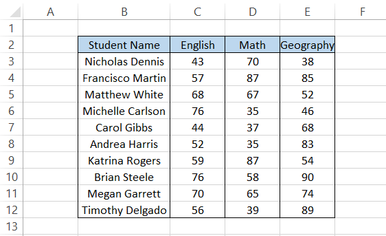
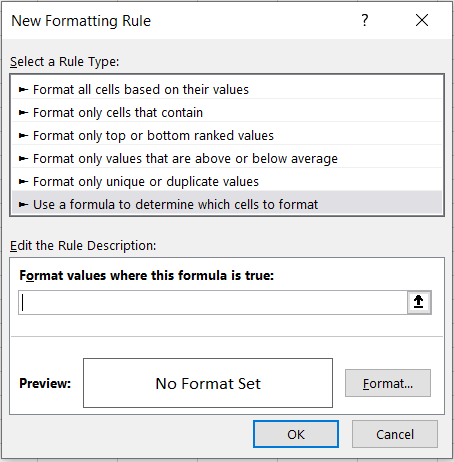
We need to highlight the minimum score on the English test. First, select the range C3:C12 and then click on the Home tab > Conditional Formatting > New Rule, which should open up the dialog box as:
Next, we set up the formula to format the specific cell, i.e., the minimum test score. The procedure will be =C3=MIN($C$3:$C$12) along with the desired cell fill.
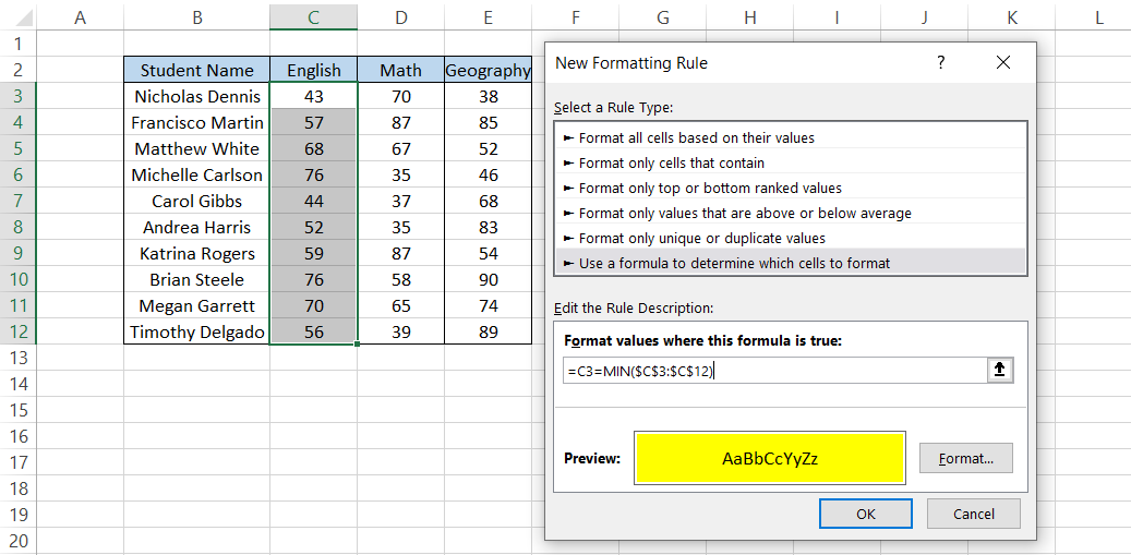
Once you click on OK, you will get the minimum value, as illustrated below:
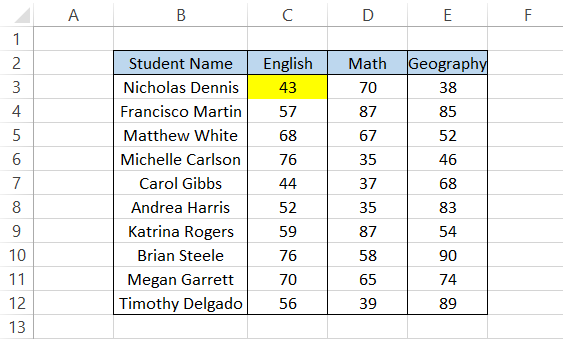
The lowest score in English is 43, as highlighted in the spreadsheet. Thus, conditional formatting makes visual analysis a lot easier and what we showed is just the tip of the iceberg.
You can also input additional conditions using IF statements to highlight minimum values based on criteria!

Free Resources
To continue learning and advancing your career, check out these additional helpful WSO resources:


or Want to Sign up with your social account?