ROUND Function
A Mathematical function in Excel that rounds up a given number to the specified number of decimal places.


What is the ROUND Function?
The ROUND function is a Mathematical function in Excel that rounds up a given number to the specified number of decimal places.
Sometimes, you might not get an exact answer in Excel using a formula or receive Excel files from clients that have numbers consisting of recurring decimal digits.
As a financial analyst, you are expected to work on many cash transactions and reconciliations, where rounding off can help you eliminate the recurring digits and keep the original number intact.
Excel only displays up to 15 digits after the decimal point when numbers are too large. After this, digits get ‘canceled,’ and you get a bunch of zeroes.
For example, the value of pi up to the first 20 digits after the decimal point is 3.14159265358979323846; however, if you use the PI function in Excel, initially, you would only get the result as 3.141593.
After shifting the formatting to include 20 digits after the decimal point, we get the result as 3.14159265358979000000.
Excel sometimes’ has its limitations in calculations, and this little exercise proves that it does its best to maintain the precision of numbers, even before we round off.
There is always a chance of getting extraneous digits in recurring numbers. This can be avoided by using the ROUND function to limit the number of digits after the decimal point.
In this article, we will see how you can use it best and take your Excel skills one step further.
-
The ROUND function is an Excel mathematical function that rounds a number to a specified number of digits.
-
Users provide two arguments to the ROUND function: the number to be rounded and the number of digits to which it should be rounded. The function returns the rounded value.
-
By default, the ROUND function uses standard rounding rules, rounding values with a fractional part of 0.5 or greater up to the nearest integer and rounding values less than 0.5 down.
-
Users can integrate the ROUND function into formulas and calculations to ensure that results are rounded to the appropriate level of precision, improving the accuracy of analyses.
Understanding the ROUND function
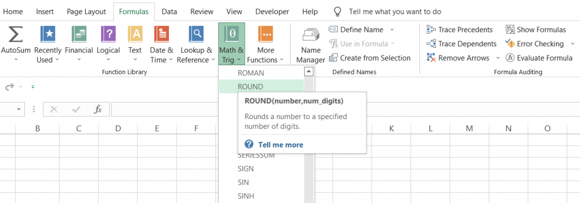
ROUND is categorized as a Math and Trigonometric function that rounds up a number to a specified number of decimal places.
The ROUND function helps you round up and round down values, depending on the decimal places in the number.
For example, if you have 17.312845 in a cell and use the function to round up the value to two decimal places, you will get 17.31. If you try to round it off to five decimal places, you will get 17.31285.
We know the ROUND function helps to round off numbers to the required number of digits, but how exactly does it work?
When the digit to the right of the final digit included in the rounded number is between zero and four, the function rounds down the value. For example, if you have 3.14159265 and round off to two decimal places, you will get 3.14.
Since the next digit (1) lies between zero and four, the value rounds down.
Similarly, the function rounds up if the next digit to the right is between five and nine. Using the process, if the number 3.14159265 is rounded off to four decimal places, you will get 3.1416 in Excel.
Thus, the function can round a number in Excel to the left or right of the decimal point, depending on the input for the num_digits argument.
ROUND function Formula
The syntax for the ROUND function
=ROUND(number, num_digits)
where,
- number = (required) the number which will be rounded to specified decimal places
- num_digits = (necessary) the number of decimal places to which you want to round the value.
Note
The num_digits argument can take negative, zero, and positive arguments to return a rounded value.
How to use the ROUND Function in Excel?
Suppose that you have several decimal numbers, as illustrated in the spreadsheet below:
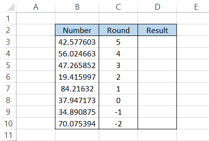
Since we have six digits after the decimal point in most numbers, we will round the numbers off to five, four, three, and so on to see how each value changes.
The formula used in cell D3 is =ROUND(B3, C3), giving us 42.5776. After dragging down the formula to cell D10, we will get the following result:
| Number | Round | Result | Explanation |
|---|---|---|---|
| 42.577603 | 5 | 42.5776 | The fifth value is 0 while the succeeding value is 3, so the value rounds down to 42.57760 or just 42.5776 |
| 56.024663 | 4 | 56.0247 | The fourth value and succeeding value both are 6, hence the value rounds up to 56.0247 |
| 47.265852 | 3 | 47.266 | The third value is 5 and the succeeding value is 8, hence the value rounds up to 47.266 |
| 19.415997 | 2 | 19.42 | The second value is 1 and the next value is 5. Here, the value rounds up to 19.42 |
| 84.21632 | 1 | 84.2 | The first value is 2 while the next value is 1. Since 1 lies between zero and four, the value rounds down to 84.2 |
| 37.947173 | 0 | 38 | The first value after the decimal is 9, so our value rounds up to the integer 38 |
| 34.890875 | -1 | 30 | Since the value in the one's place (before the decimal) lies between zero and four, our value rounds down to 30 |
| 70.075394 | -2 | 100 | Since the value the in ten's place (before the decimal) lies between five and nine, our value rounds up to 100. |
As you can see, based on the value of the digit after the final digit is included in the rounded number, the final value is either rounded up or down.
If the digit after the final included digit lies between zero to four or five to nine, you get a number that is either rounded down or rounded up.
This means it assumes a logic of n + 1 for rounding off numbers in Excel. So, if you need to round off a number to the third value, the fourth digit after the decimal is important to determine whether the value will round up or down.
However, the same cannot be said when you use a negative integer for the num_digits argument.
The logic here changes to n for rounding off the numbers in Excel. So, if you need to round off a number to -2 and the number is 32.4, since the 3 (two digits before the decimal) lies between zero and four, you will get 0.
Rounding off without the ROUND function
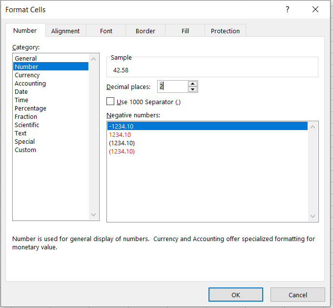
If you are still unsure how to use the ROUND function, there is a little hack that you can use in Excel to round off numerical values. It's none other than the format cell dialog box.
To open the format cell dialog box in Excel:
-
Select the cell containing the number and press Ctrl + 1, the keyboard shortcut
-
Click on the 'Number' category or 'Currency' if you are rounding currencies.
-
You can shift decimal places from zero to thirty using the spin button. However, the only downside to this method is that you can't shift the decimal places toward the left using negative numbers (e.g., -1, -2, etc.)
-
Once done, click on OK.

ROUND Function examples
Let's take a look at some of the practical examples below.
Example 1
As a financial analyst, you will be working on many files that consist of interest rates and monetary transactions, such as buying and selling bonds and equities and M&A and LBO deals.
Sometimes, when you receive transaction files from a third-party website or client, there might be a rounding-off issue for interest rates and the amounts.
These are minute issues not even worth raising with the clients or even your own IT team, which is why making use of the ROUND function makes even more sense.
For example, 4.16% will be represented as 4.1576487984935%, while $35,868 may be represented as $35,868.0006848.
Assume that you have the interest rates and the amounts illustrated below:
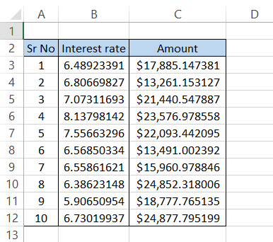
All you need to do is use the formula =ROUND(B3,2) in column D and =ROUND(C3,2) in column E, respectively, to get the rounded-off values:
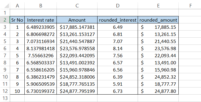
Once the values are in a proper format, it makes working in Excel all the easier!
Example 2
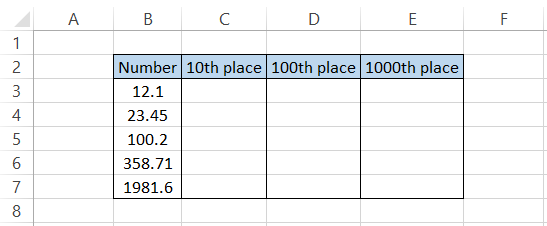
Rounding a number to the desired number of decimal places is easy, but can you do the same to the nearest 10/100/1000th position?
What numerical inputs do you need to add to the function?
Suppose that you have the following numbers in Excel:
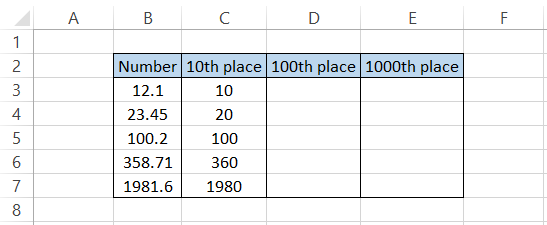
To round the number to the nearest 10, we will use the formula =ROUND(B3,-1), which gives us the following result:
Similarly, to find the nearest 100 and 1000, we will use the formula
=ROUND(C3,-2) and =ROUND(C3,-3) respectively. This will provide the following results:
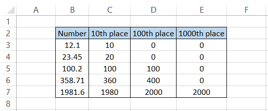
This way, using a negative integer for the num_digits argument, you can easily find the nearest 10/100/1000, respectively.
ROUND function vs. ROUNDUP function
You can use alternatives for the ROUND function in Excel, but they fulfill different purposes.
An important feature that distinguishes these functions from ROUND is that they do not follow the standard rounding rules, i.e., when the 'nth' digit (the digit to the right of the final digit included) lies between 1 to 4, then the number rounds down, whereas, when the 'nth' digit is between 5 to 9, the number rounds up.
The first of those two functions is ROUNDUP, categorized as a Math and Trig function. It rounds a numerical value away from zero.
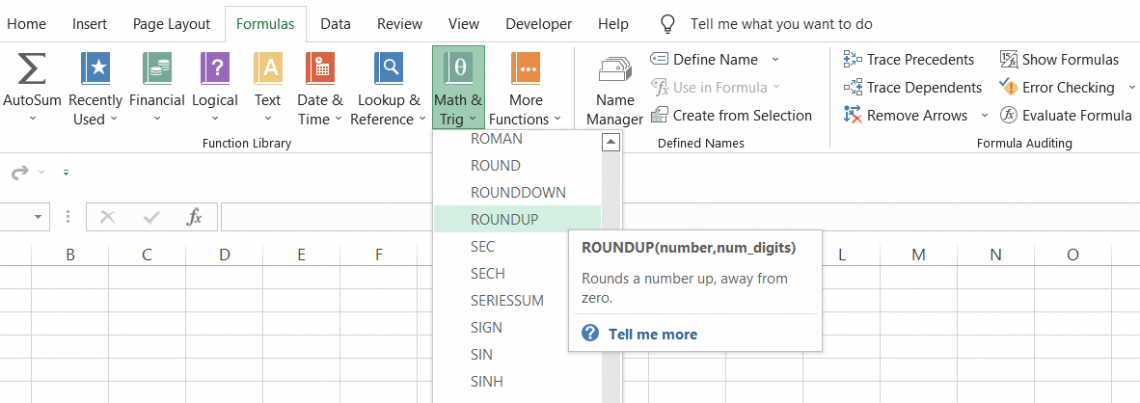
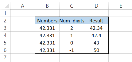
What the function does is irrespective of the 'nth' digit, the function always rounds up the value. For example, 42.331 rounded up to different decimal places provides the following results:
The syntax for the function is:
=ROUNDUP(number, num_digits)
where,
- number = (required) the number which will be rounded up to the specified number of digits after the decimal
- num_digits = (required) the number of decimal places that you want to round up the value to
Suppose that you have the data illustrated below:
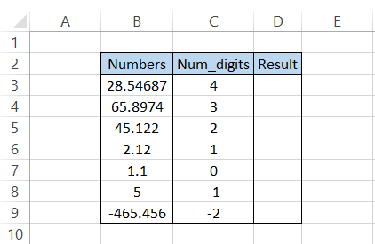
By using the formula =ROUNDUP(B3, C3) in cell D3 and dragging it down to the last cell, we get the following result:
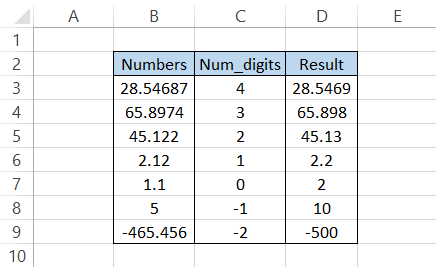
As you can see, the numerical value gets rounded up irrespective of your number at the 'nth' digit position, as illustrated in the example above.
ROUND function vs. ROUNDDOWN function
The other function that ignores the standard rounding-off rules is the ROUNDDOWN function. It works opposite to that of the ROUNDUP function.
ROUNDDOWN is categorized as a Math and Trig function. It reduces the 'nth' decimal number by rounding it towards zero.
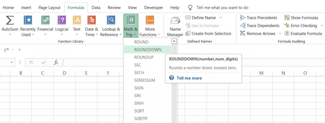
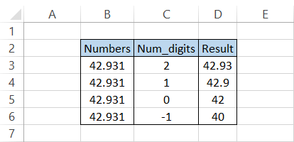
When you use the function, no matter what number you have at the ‘nth’ digit position, the result will always be a numerical value rounded toward zero. For example, if you have 42.931, the results rounded to different decimal places are:
The syntax for the function is:
= ROUNDDOWN(number,num_digits)
where,
- number = (required) the number which will be rounded to specified decimal places
- num_digits = (required) the number of decimal places that you want to round the value down to
Suppose that you have the interest rates in Excel illustrated below:
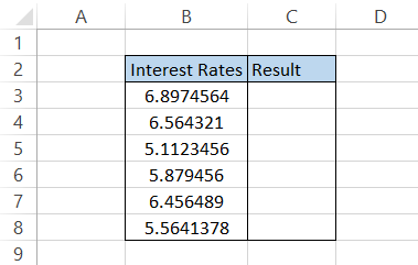
If you want to limit the rates to just two decimal places, you can use the formula =ROUNDDOWN(B3,2), which should return the following:
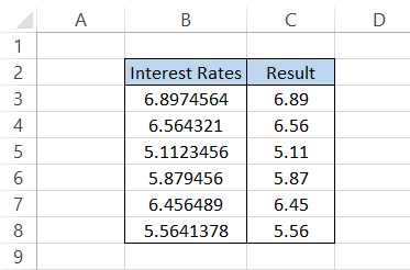
The formula will return only two digits after the decimal point, even if there are more in the original numerical value, as shown in the example above.
Each function has its pros and cons, so it’s necessary to decide the situations to use each, as they can return conflicting results!

Free Resources
To continue learning and advancing your career, check out these additional helpful WSO resources:


or Want to Sign up with your social account?