Alphabetize in Excel

How to Alphabetize in Excel?

Alphabetize means alphabetically arranging your data from A - Z or vice versa. Alphabetize is one of the easiest tasks to perform in Excel. Arranging the values can be done alphabetically for text and ascending or descending for numbers.

Some of the methods to Alphabetize in excel are: 

• Sort
• Filter
• Sort Formula (Excel 365)
• COUNTIF And VLOOKUP
• Combination Of INDEX-MATCH, ROW, COUNTIF, IF & IS Functions

This article will illustrate each of these methods to organize your data alphabetically.

Sort

Sort functions help to sort the values in ascending or descending order. You can find the sort function in two different places in Excel - the data tab and the home tab.

1. Sorting from Data Tab

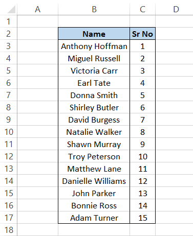
Assume that you have the following data consisting of employee names working in your organization:

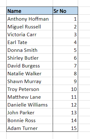
The data tab is the first place to find the dedicated Sort function. First, select the data you need to sort, i.e., range B3:C17, then click on the Data tab, leading you to the Sort function in the Sort and Filter section.

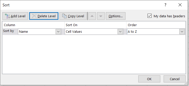
This will open up a dialog box where you will get the option to sort the data by different column names and order (A to Z or Z to A), in which the sort function will arrange the data in the spreadsheet.

You can also use the keyboard shortcut of Alt + A + SS to open this window in Excel. We have decided to alphabetize the data as per the ‘Name’ column in ascending order.

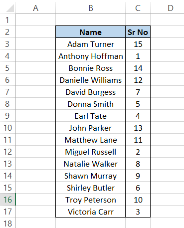
When you click on Ok, the data in your spreadsheet will look like this:

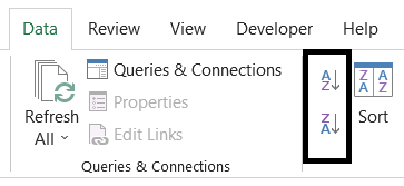
If you feel that selecting those parameters in the dialog box can be confusing for a simple alphabetizing task, click on the Data tab to find two icons beside the Sort function.

The one on the top will rearrange your data in ascending order, while the one on the bottom will regroup the data in descending order. You can also use the keyboard shortcut of Alt + A + SA to arrange data as A - Z or Alt + A + SD as Z - A.

2. Sorting from Home Tab

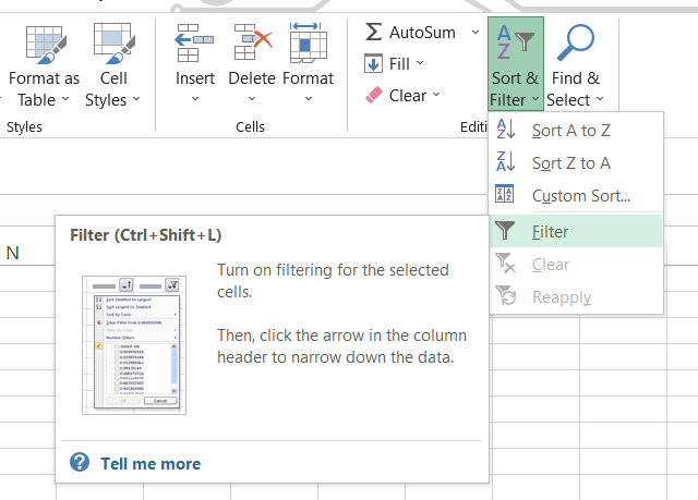
Another way you can sort the data in either A - Z or Z - A format is by clicking on the Home tab, where you will find the option to Sort & Filter.

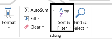
Select the data which you need to rearrange in the spreadsheet. Next, click on the home tab, and then on the Sort & Filter dropdown will show you the options to ‘Sort A to Z’ or ‘Sort Z to A’.

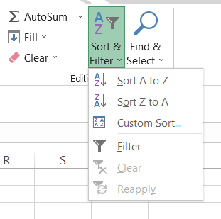
This way, Excel will instantaneously alphabetize your data in a matter of seconds. You can also use the keyboard shortcut of Alt + H + S + S to rearrange data in ascending order or Alt + H + S + O for descending order. Finally, Sort is a function in Excel where you are spoilt for choices! 

Filter

Similar to the Sort, you can find the Filter function in two different places - the Home tab and the Data tab. First, select the data you need to rearrange and then click on the data tab to find the option to Filter. You can also use the keyboard shortcut of Alt + A + T to filter data. 

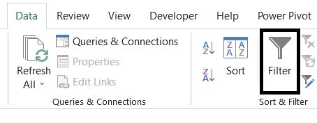
You will notice dropdown arrows on the headers of your data tables. Either click on it or press the down arrow key on the keyboard as it will reveal the following options to you:

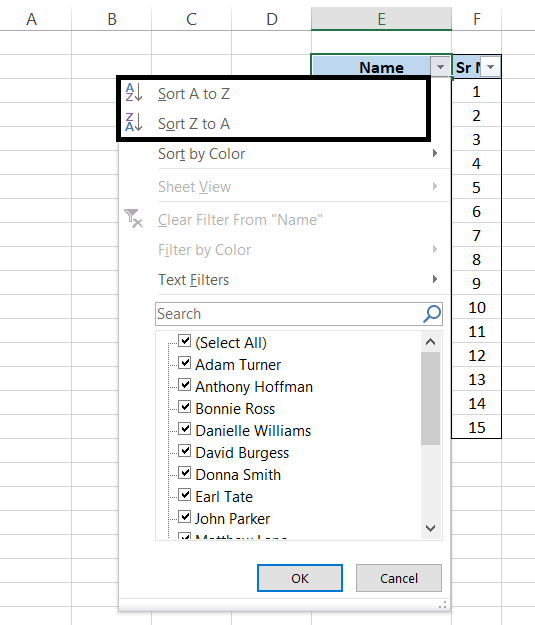
The first two choices are about alphabetizing your data in Excel either in A - Z style or Z - A style. Another way you can filter the data to rearrange it is by clicking on the Home tab and then on Sort and Filter to find the option to filter.

It will display similar dropdown arrows on the header on the data from where you can rearrange the data in ascending or descending order. After selecting the data to add filters, you can also use the excel shortcut key of either Ctrl + Shift + L or Alt + H + S + F.

Sort Formula (Excel 365)

One of the newest additions (not so new anymore) to Excel is using Sort as a part of the formula in an Excel spreadsheet. The formula then sorts the referenced range in ascending or descending order.

The result obtained by the formula is a dynamic array of values that is of the same shape as the provided array argument and usually ‘spills’ into a range in the spreadsheet.

The syntax for the SORT function is:

=SORT(array, [sort_index], [sort_order], [by_col])

where,

• array = The range that needs to be sorted. This is a required parameter.
• sort_index = Indicates which row or column to sort by. This is an optional parameter.
• sort_order = Indicates the order to sort the data where 1 indicates ascending order(default value) and -1 indicates descending order. This is an optional parameter.
• by_col = A boolean value indicating the direction to sort the values by. The FALSE value sorts the data by row(default) while the TRUE value by column.

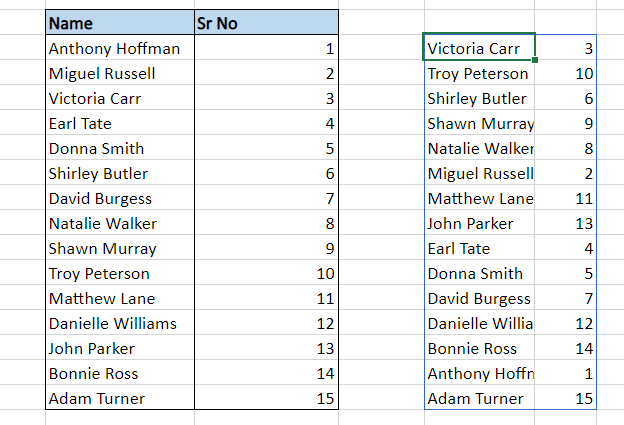
Let us take a look at an example of SORT Function. Assume that you have the following data consisting of employee names working in your club:

You will use the formula as =SORT(B3:C17, 1, 1, FALSE) in any of the cells (you don't need to drag down the formula) which will give you the result as:

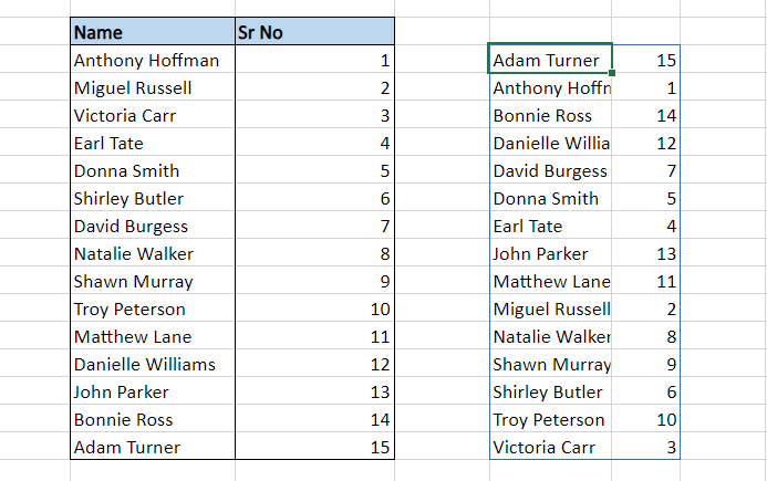
After breaking down the formula, we see that the sort_order parameter as 1 rearranges the data in ascending order for column ‘Name’.

If we had wanted the data in descending order, we need to change the value of the third parameter to -1 such that the formula becomes =SORT(B3:C17, 1, -1, FALSE) and the result that you will get is:

COUNTIF and VLOOKUP

The combination of COUNTIF and VLOOKUP functions is a powerful tool to alphabetize your data in spreadsheets. We will try to break down the formula into two parts.

The first part is made of the COUNTIF formula, where you reference the range and create a sorting order, i.e., whether you want to sort the data in either ascending or descending.

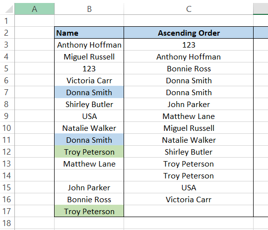
The formula that you will use in a separate column created is =COUNTIF($B$3:$B$17, “<=” & B3), which will give you the result as:  

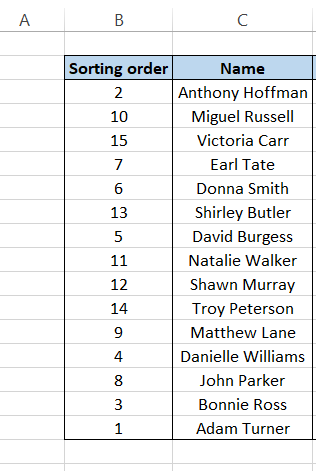
This creates an index for our data under the column header ‘Name’. So if this data would be arranged in ascending order, then the first value would be 1, followed by 2, and so on. Next, to arrange the values in A - Z order, we will use the VLOOKUP function.

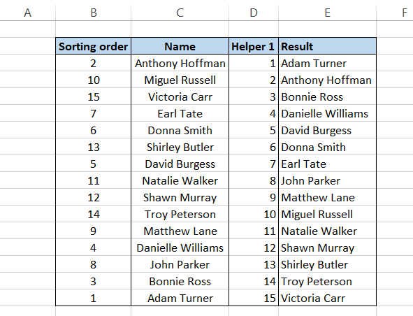
We create a helper/reference column for number series besides the ‘Name’ column and use the formula in column E as =VLOOKUP(D3, $B$3:$C$17, 2, FALSE) to give the result in ascending order.

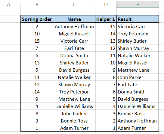
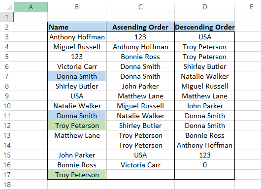
Now, if you want the same data in descending order, all you need to do is reverse the values in the ‘Helper 1’ column such that your result becomes:

Remember, if there is an alternative method in Excel to use a specific function, it is mainly due to its limitations in traditional functions. For example, what you can achieve with formulas is far more than what can be done with the functions located in the Excel ribbon.

Combination of iNDEX-MATCH, ROW, COUNTIF, IF & IS Functions

This is the most challenging method in this article due to the complicated formula involved in finding the value in ascending or descending order. However, it is a vital formula having practical usage while working on Excel versions 2019 and below (you can still use the formula in Excel 365 instead of the SORT formula). 

The formula that you will be using in the cell is: 

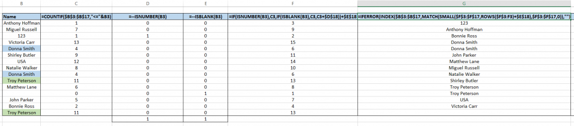
=IFERROR(INDEX($B$3:$B$17, MATCH(SMALL(NOT($B$3:$B$17 = "") * IF(ISNUMBER($B$3:$B$17), COUNTIF($B$3:$B$17," <= "&$B$3:$B$17), COUNTIF($B$3:$B$17, "<=" & $B$3:$B$17) + SUM(--ISNUMBER($B$3:$B$17))), ROWS($B$3:B3) + SUM(--ISBLANK($B$3:$B$17))), NOT($B$3:$B$17 = "") * IF(ISNUMBER($B$3:$B$17), COUNTIF($B$3:$B$17, "<=" & $B$3:$B$17), COUNTIF($B$3:$B$17, "<=" & $B$3:$B$17) + SUM(--ISNUMBER($B$3:$B$17))), 0)), "")

which will give you the following result: 

We understand this formula is incredibly complicated. So let’s break it down into different parts and get the result that we will later concatenate into the final formula we have used.

The first part of the formula is =COUNTIF($B$3:$B$17, “<=” &B3) which returns the index number of the value in column B. If these numbers are arranged in ascending or descending order, they will give you the result for A - Z or Z - A sorting in Excel. The table will return the following values after using the formula:

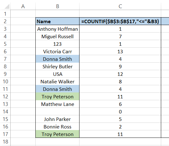
Some important things to note are:

• If column B has duplicate values, the formula will return the same number (e.g., Donna Smith).
• The formula will return the number like 0 in case of blanks.
• In the case of numbers and text, numbers starting from 1 are assigned to both the series since both the values are processed side by side(for example, 123 and Anthony Hoffman both are the beginning values of their respective series and hence are assigned the value 1).

The next part of the formula uses the functions ISNUMBER and ISBLANK, which return the value as TRUE if the value is either a number or a blank cell, or else it returns as FALSE. We will, however, use the double negative before the formula that returns the result in terms of 1(TRUE) & 0(FALSE).

The formula used is = --ISNUMBER(B3) and = --ISBLANK(B3) in columns D & E, respectively, to get the result as:

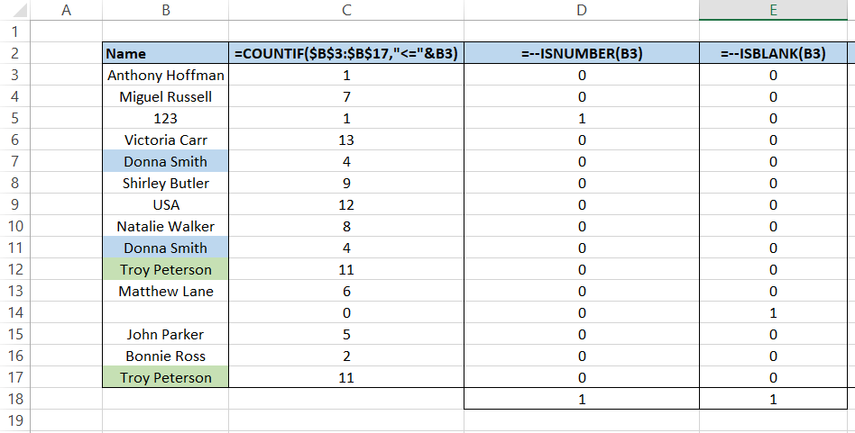
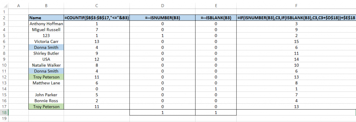
In cells D18 and E18, we obtained all the values in range D3:D17 and E3:17, respectively, using the SUM function. Next, we make another column where we will be using the formula =IF(ISNUMBER(B3), C3, IF(ISBLANK(B3), C3, C3+$D$18)) + $E$18, which performs three different tasks:

• If the value is blank, the formula returns as zero (for value in cell B14, the formula returns a value of 0).
• If the value is a number, it returns the corresponding number in column C and adds the total number of blank cells present in cell E18 to the number (for value in cell B15, i.e., 123, the result returns as 2).
• If the value is text, it returns the value in column C and the sum of all numerical values and blank values in cell D18 and E18 (for value in cell B6, i.e., Victoria Carr, the value returns as 15).

And here comes the final part.You will be using the formula =IFERROR(INDEX($B$3:$B$17, MATCH(SMALL($F$3:$F$17, ROWS($F$3:F3) + $E$18), $F$3:$F$17, 0)), "") which will give you the final result of data in ascending order.

The formula MATCH(SMALL($F$3:$F$17, ROWS($F$3:F3) + $E$18) acts as a lookup value which usually returns a result that is higher than the sum of blanks represented by cell E18. As a result, if there are any blanks in your spreadsheet, they will be represented at the end of our range.

When you combine all these formulas considering the value of SUM of blanks and numerical values without any helper columns, the result is an array formula that directly arranges your range in ascending or descending order. Since it is an array formula, press Ctrl + Shift + Enter to get the result in the cell.

Alphabetize ExampleAlphabetize in Excel Example

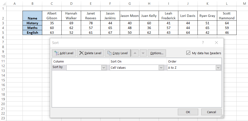
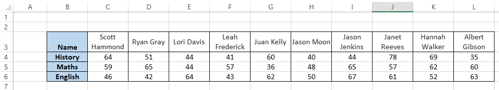
Suppose that you have the marks scored by students in three different subjects - History, Maths & English in a horizontal table. If you need to alphabetize the data, open the Sort function using one of the keyboard shortcuts of Alt + A + SS. 

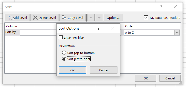
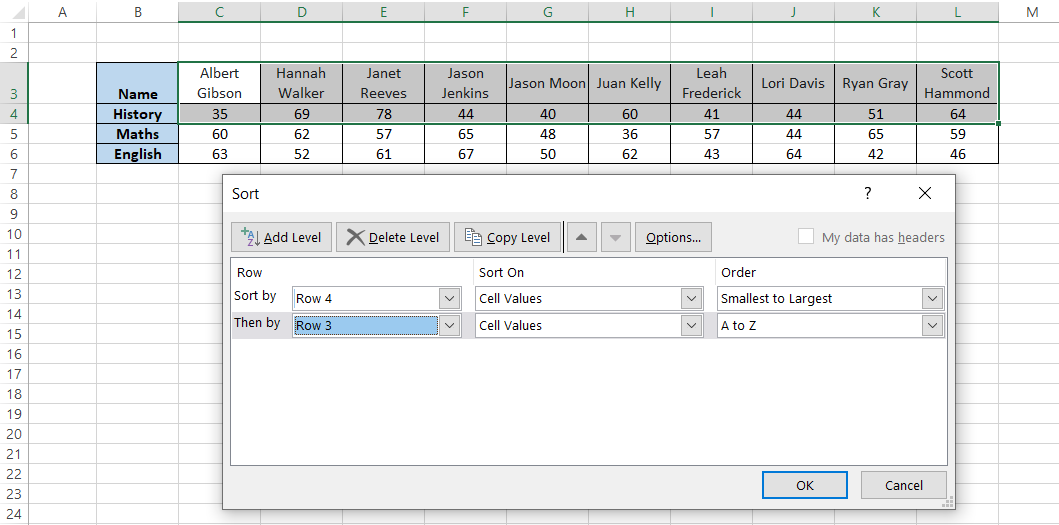
Now go into Options and select the orientation as ‘Sort left to right’. Press Ok.

Here we will sort our data by ‘Name’ row, which is Row 2 in the dropdown menu, and keep the order as Z to A. Then, when you click on Ok, you will get the result as:

Multi-level parameter for the sort function sorts one range of data with reference to another data. 

If you press Ok and run the logic, you will get the following result: 

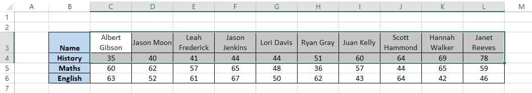
Do you notice that all the values are first arranged in ascending order for row 4, and in reference to those values, the values in row 3 are arranged. For example, ‘Jason Moon’ and ‘40’ were in cells G3 & G4, respectively.

After sorting the number from smallest to largest, the value ‘Jason Moon’ also switched places along with the number. In this way, the multi-level Sort lets you alphabetize data in more than one referenced column.

Alphabetize Common Errors

This may not be an error but rather a warning that Excel displays based on the data we select to sort. For example, most of the time, we may select only the row that we want to rearrange in ascending order to get this error: 

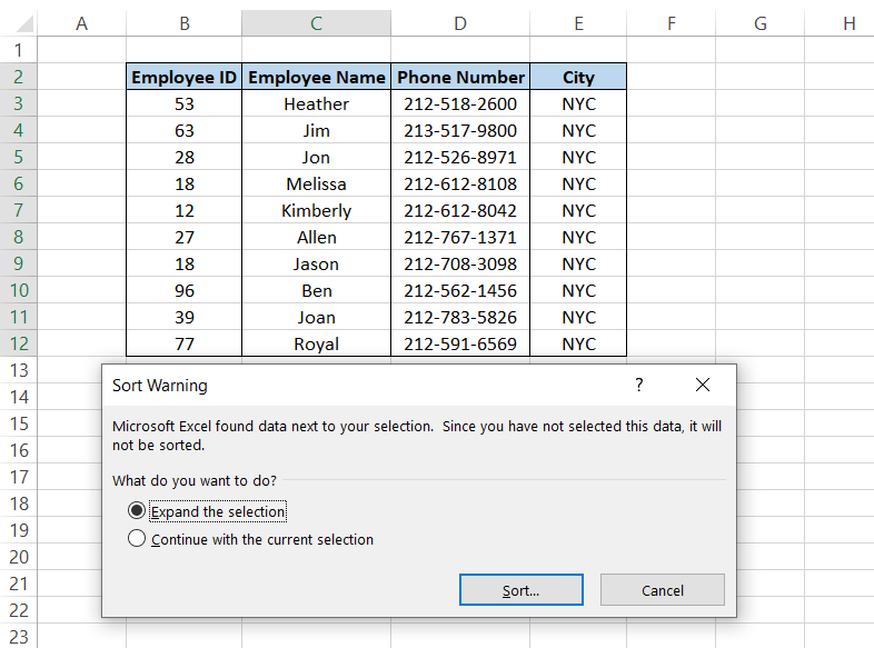
This option lets you go with two alternatives:

• Sort the entire table based on the selected data range by choosing the option ‘Expand the selection’. So assume that if the value ‘Heather’ in cell C3 goes to the last cell i.e., C12, all the corresponding cell values of B3, D3 & E3 will take the position in B12, D12 & E12 besides the value ‘Heather’.
• Sort only the column you have selected while other data remains static by choosing the ‘Continue with the current selection’ option. This only sorts the data in column C, and all the values in the rest of the column remain the same.

More on Excel

To continue your journey towards becoming an Excel wizard, check out these additional helpful WSO resources.

• Advanced Excel formulas you must know
• Developer tab
• Excel keyboard shortcuts for Windows and Mac
• Excel modeling best practices
• INDEX MATCH formula in Excel