Excel Consolidate
A built-in Excel feature/function that allows you to summarize and aggregate data from multiple separate worksheets into one summary worksheet.


What is Excel Consolidate?
Excel Consolidate is a built-in Excel function that allows you to summarize and aggregate data from multiple separate worksheets into one summary worksheet. Multiple separate worksheets can be either located in one or different workbooks.
Excel offers two methods to consolidate the data:
- By Position: It applies to source data that has the same order and labels. This method is commonly used to aggregate data obtained from multiple sources that use one universal template.
- By Category: It applies to the source data with the same labels but in a different order. This method is commonly used to aggregate the data which was obtained from multiple sources that use an individual template but the same data labels.
Note
Consolidation of data by category is like the construction of the Pivot Table but with less flexibility in terms of reorganization of categories.
The Consolidate Excel function is a helpful tool for financial professionals, especially those who aggregate data.
More specifically, it can be used by the auditors to consolidate data provided by the client and by the reporting professionals to consolidate information obtained from different entities within the group, etc.
- Excel Consolidate is a feature in Microsoft Excel that allows users to combine data from multiple ranges or worksheets into a single summary.
- Consolidate is useful for aggregating data from different sources or organizing information spread across multiple sheets into a cohesive view.
- The purpose of Excel Consolidate is to combine data, summarize information, and simplify analysis through a unified view which makes it easy to identify patterns, trends, and any discrepancies.
- The best practices of Excel Consolidate start with organizing source data, choosing appropriate functions, and regularly updating data.
Excel Consolidate: How to Consolidate the Data
As previously mentioned, there are two methods to consolidate data in Excel – by position or by category.

Having said that, you don’t choose the consolidation method. Excel does that automatically based on the data range you specify and the arrangement of the consolidating worksheets.
Before you proceed with data consolidation, you have to arrange it in labeled rows and columns (blank rows and columns should be removed). An example below will provide you with step-by-step instructions on how to consolidate the data in Excel.
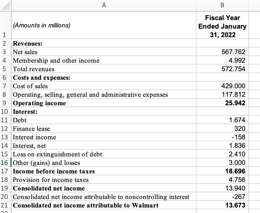
Let’s assume that we want to consolidate Walmart’s income statement for the three-year period.
Step 1: Open an Excel workbook.
Step 2: Make sure that the collected data is arranged in a way that can be further used in consolidation. In other words, rows and columns are clearly labeled, and the worksheets that will be used for consolidation purposes are clearly identifiable.
In this example, we have collected the company's income statement for a three-year period. As seen below, each year’s income statement was placed on a different worksheet.

Step 3: Create a blank worksheet that will be used for consolidation purposes (for example, a worksheet called “Consolidate”), as seen in the image below.

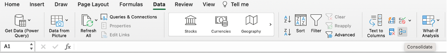
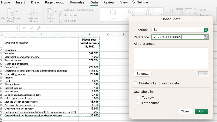
Step 4: Press on any cell in the worksheet created for consolidation purposes, select the Data tab located on the ribbon at the top of an Excel workbook, and choose the Consolidation button, as shown below.
Step 5: Once the Consolidation button is pressed, the following window pop-ups and the terms figuring in it are explained below:
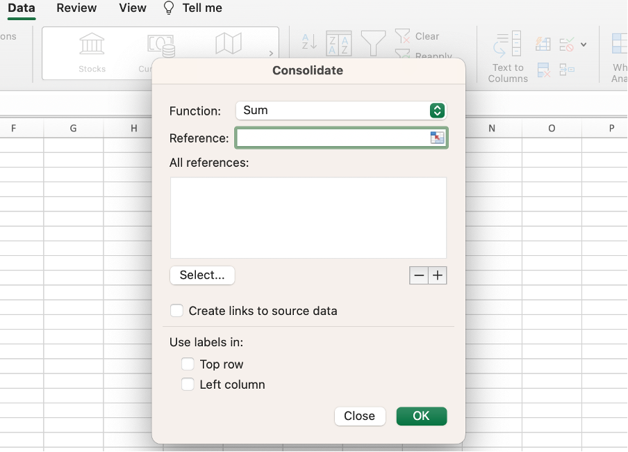
- Function: refers to the method of consolidation (sum, average, product, etc.).
- Reference: refers to the data range to be consolidated, including labels. If the data range is located in another workbook, click on Select to locate the appropriate workbook. Once found, select OK, and Excel will enter the file path.
- Create links to the source data: This function creates links to the worksheets containing data, which allows automatic updates in case of any changes in the referenced data.
- Use labels in: provides an option to include labels into consolidated data.
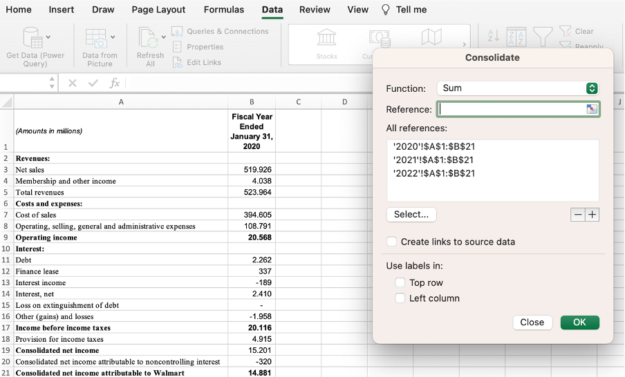
Step 6: Select the data range and press the plus button “+”.
Step 7: Repeat the same step for each worksheet that contains data that needs to be included in the consolidation.
Step 8: Check the respective boxes if you want the final result to show links to source data or display labels. This step is optional.
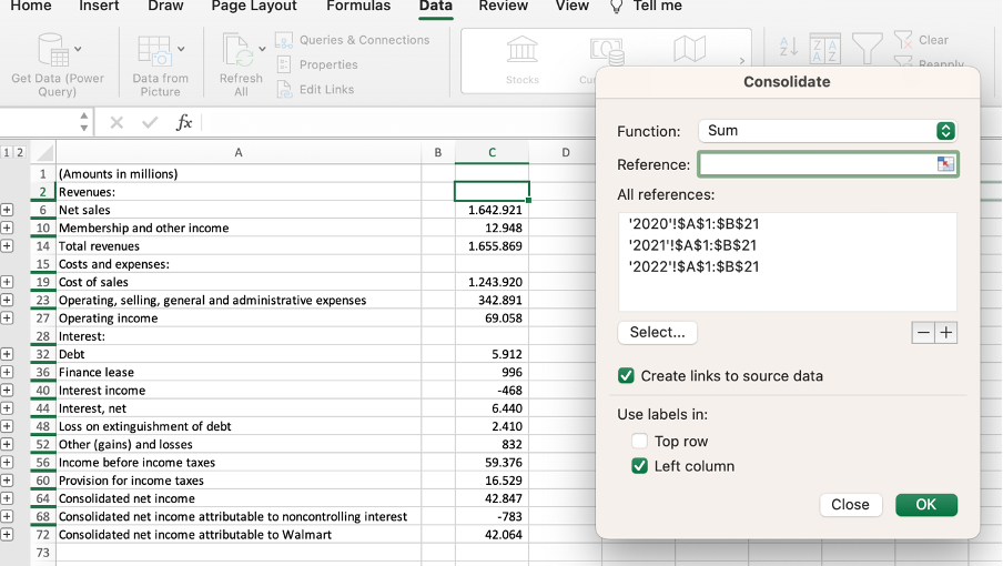
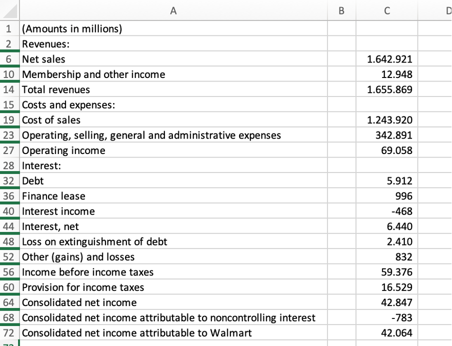
Step 9: Press the OK button and get the consolidated result.
If you want to change the reference, you will have to update the Consolidate pop-up reference field. Once you make the respective changes, simply press the OK button to get the new result.

Free Resources
To continue learning and advancing your career, check out these additional helpful WSO resources:


or Want to Sign up with your social account?