Basic Excel Formulas

Basic Excel Formulas Guide

At the core of Excel's functionality lies its extensive library of formulas, which enable users to perform a wide range of mathematical, statistical, and logical operations on their data.

Excel formulas are mathematical equations for calculations, data manipulation, and analysis. When a formula is typed into a cell, it shows up in the formula bar, which gives a detailed view. Thus helping the users to edit the formula, make corrections, and fix the errors.

Excel formulas helps us to perform variety of tasks ranging from basic arithmetic calculations to complex data analysis and financial modelling

Basic Excel Formulas Guide aims to provide a fundamental understanding of some of the most commonly used Excel formulas, making it  accessible to beginners while also serving as a quick reference  for more experienced users.

We will cover some essential formulas such as SUM and AVERAGE for basic calculations, as well as IF statements for conditional logic. You'll also learn about functions like VLOOKUP and HLOOKUP for data retrieval and CONCATENATE (or CONCAT) for combining text. 

This guide will give you an overview of important Excel formulas that you can use in your respective jobs.

What is an Excel function?

An Excel function is a predefined expression that performs mathematical, logical, financial, and statistical operations using user input values as the argument. 

If you are a beginner with absolutely no knowledge about what different functions you can use, head over to the Formulas tab and check out the different functions that are available in the Functions Library. 

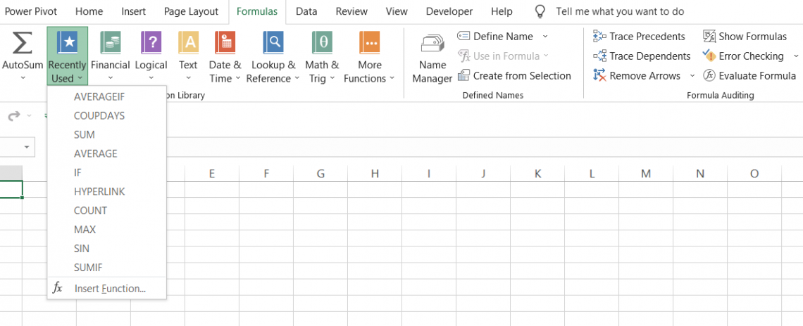
Let’s say you need to find the sum of the numbers 5, 10,15, 20, and 25. The steps you need to follow to get the result via Excel function are:

• Select the cell in which you want the result and click on Formulas > Math & Trig > SUM

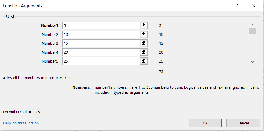
• Input the values as the arguments in the dialog box that opens.

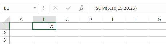
• Click on Ok. You will get the result as 75 as the addition of (5 + 10 + 15 + 20 + 25) in the spreadsheet.

Microsoft has a complete dictionary for all the cool functions that you can use in Excel.

What is an Excel formula?

An Excel formula is an expression of the Excel function, such as SUM, AVERAGE, IF, etc., that operates to return results based on the reference of a cell or range of cells.

Let's just agree to the fact that absolutely no one goes into the Formulas tab, then click on More Functions, select Statistical from the drop-down menu to select the AVERAGE function to find the average of values in the spreadsheet. 

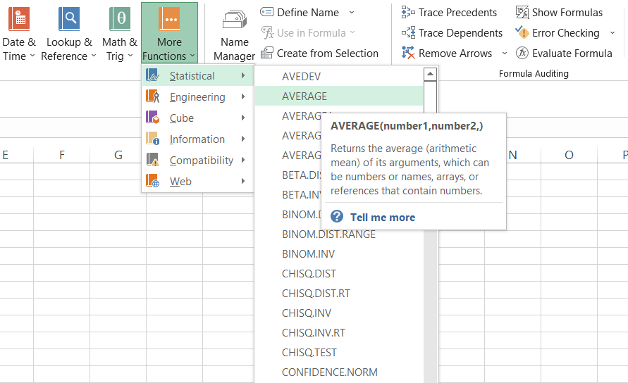
Yes, you might apply this method to check the different functions you can use for data analysis, but the most preferred method of using different functions in Excel is the use of equal sign(=) in a cell followed by the function you intend to use.

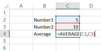
So if you need to find the average of n numbers in the spreadsheet, the formula that you will be using will be 

=AVERAGE(Number1,[Number2]...)

Thus, Excel formulas and functions perform different tasks in seconds and improve your work efficiency. We will go ahead and see different formulas you can use, even as a beginner.

Basic Excel formulas

Excel will give you a variety of formulas and functions depending on what you intend to achieve from the given dataset. It can be finding the sum of ten numbers, the average of five numbers, counting how many numbers are greater than five, or simply returning a value from the n column based on the lookup value.

The different formulas that you can use in Excel are:

SUM

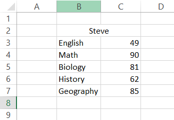
The SUM function will calculate the sum of all the values in the selected range of cells. It will add all the values in a cell or range of cells to give you the result in which you use the formula. For example, given below are the marks scored by Steve in his examination.

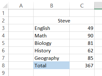
By using the formula =SUM(C3:C7) in cell C8, we can get the total marks scored by Steve in his exams as 367. Alternatively, you can add individual cell values in the formula such that the formula becomes =SUM(C3, C4, C5, C6, C7). The latter gives you the flexibility to skip a particular value to find the sum of a range of cells.

Another way you can use the sum function is by pressing the Alt + equal sign(=) in cell C8, also called the AUTOSUM function.

Check out our article on AUTOSUM to learn more!

AVERAGE

The AVERAGE function returns the average for the range of cells. For example, if you need to find the average of the marks scored by Steve in his exams, you just need to type the formula in the cell as =AVERAGE(C3:C7) to give you the result as:

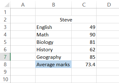
So instead of finding the SUM for all the numbers and then dividing it by the number of values, i.e., 367/5, the AVERAGE function gives you the mean or the average of the range of cells by referencing the values in the formula.

COUNT

The COUNT function does exactly what it sounds like: it counts the number of cells in a range that contain a numerical value. It ignores any cell that contains text or data that is non-numeric. It will also ignore empty cells. 

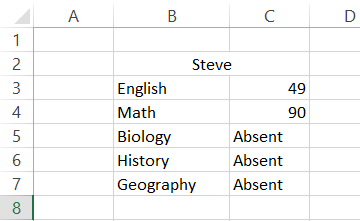
Here’s an example. Assume this dataset below shows Steve’s grades for five subjects. Steve is also not a good student; he skipped three exams.

From the data, you are looking to find out how many exams Steve completed.

The appropriate formula to find out how many exams Steve completed is as follows: s =COUNT(C3:C7) 

This gives the following result:

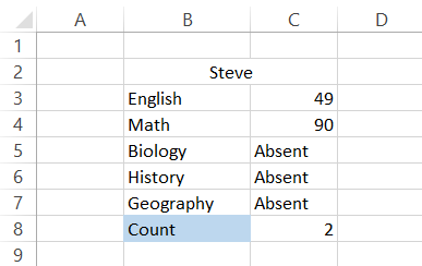
As you can see, the COUNT function ignores the cells C5, C6, and C7 in the result as they are text-based and gives the result as 2. Do note that this method of counting cells will only work on cells containing numerical values.

MODULUS

The MOD function returns a remainder when you divide a particular number with a divisor. Suppose that you have three numbers 10,13, and 25.

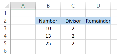
 If you need to check what numbers are divisible by 2, you will use the formula =MOD(B3, C3) in the cell D3 to give you the result:

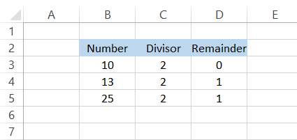
If the remainder is equal to zero, then our number is divisible by 2. For number 13, the remainder returns as one since 2 x 6 give 12, and 1 is added to give the result as 13. The MOD function has its application in the calculation of every nth value in the spreadsheet 

You can read more about the MOD function here.

POWER

The POWER function is an alternative to the exponent operator ( ^ ) that returns a result for a number raised to a certain power. For example, if you need to find the result for 8 to the power of 3, the formula you will use is =POWER(B3, C3) to give you the result 512.

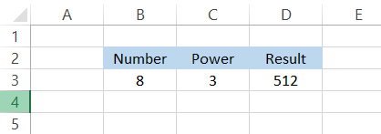
You can also write the formula as = POWER(8,3) by hard coding the value of power and the number. The other alternative that would give you the same result is the use of an exponent operator such that the formula becomes =B3^C3. Every method has its advantages and plays different roles in complicated formulas.

CONCATENATE

The CONCATENATE is one of the most underrated functions in Excel. By using it as a formula, you can join several strings in different cells into one string. For example, the values for cells B2, C2, and D2 are ‘Welcome,’ ‘to,’ and ‘WallStreetOasis,’ respectively. 

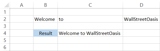
By using the formula = CONCATENATE(B2, C2, D2), you will get the entire string as ‘Welcome to WallStreetOasis’ in a single cell C4. Another alternative that you can use to CONCATENATE is the use of the ampersand (&) symbol between the strings that are inside the quotation marks.

Using the ampersand (&), the formula in C4 becomes = B2&C2&D2 which will give you the same result.

 LEN

The LEN formula(Length) will return the total number of characters for the referenced text string. If you need to find the number of characters in the word ‘Welcome to WallStreetOasis’ in cell C4, you will use the formula =LEN(C4) or =LEN(“Welcome to WallStreetOasis”). 

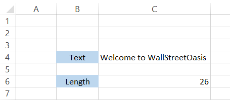
The formula returns the result as 26, meaning there are 26 characters in total inside the text string in cell C4. But wait! If you count the letters manually, it only makes up to 24 characters. Where the heck did two additional characters come from?

Excel counts the space between the words as characters as well. We can see two spaces, i.e., first after the word ‘welcome’ and another after ‘to’ in the text string. This takes our total to 26 characters.

LEFT RIGHT & MID

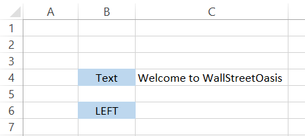
The LEFT, RIGHT & MID essentially returns characters from the left, right, or middle of the text string. For example, assume that you have the text ‘Welcome to WallStreetOasis” in cell C4.

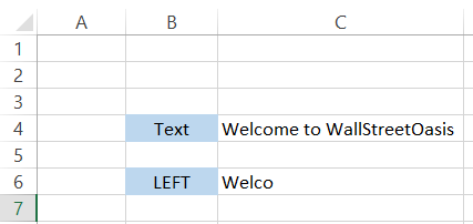
If you use the formula =LEFT(C4,5), the formula will capture the first five characters from the left and return them as a result. The first five characters from the left are ‘Welco,’ which is exactly the result we get using the formula.

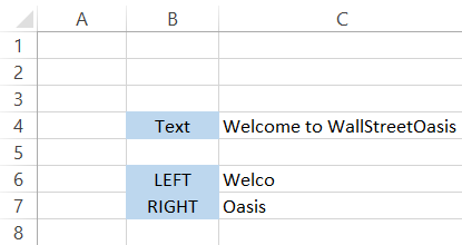
The formula =RIGHT(C4,5) will return the first five characters from the right side of the text string. So the result you will get in cell C6 will be ‘Oasis.’

The number of characters you need to return depends on you and can be changed in the formula. If you need to return six characters, the formula becomes =RIGHT(C4,6) to give you the result as ‘Oasis.’

The formula for MID takes an extra argument and the number of characters to return. It is the starting place from which you need to return the characters of the text string.

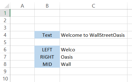
For example, by using the formula =MID(C4,12,4), the formula counts twelve characters from the left and uses it as a starting point to return four characters which are ‘Wall.’

This formula gives more flexibility in terms of returning the required characters from a text string.

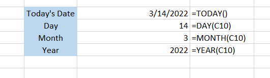
TODAY()

The TODAY function returns the current date displayed by your system in Excel. If you are unsure what today’s date is, just use the formula =TODAY() in any cell, and it will return. Forgetting the current day can be quite annoying; yes, it happens to the best of us.

But it will only work as long as your system displays the correct date. If due to some error, the date is changed or you are using a different time zone, then you might get different results.

Additionally, three important functions that go well with TODAY functions are DAY(), MONTH(), and YEAR(). As the name suggests, the three functions return the day, month, and year from the date.

If you save the excel and open it after 24 hours, you will find that our value for =TODAY() formula changes. Isn't it logical that if the day changes in the system, Excel will also reflect it? 

Hence, the TODAY formula is one of the indispensable tools of Excel.

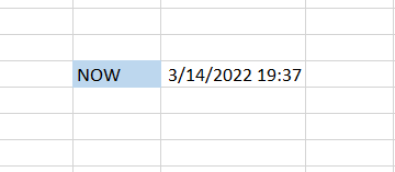
NOW()

The NOW function is similar to the TODAY function, but in addition to the date, it also displays the current time in HH: SS format. For example, if you use the formula =NOW(), the result that you will get is as illustrated below:

IF()

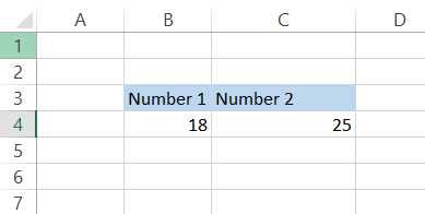
The IF function is a logical statement that checks the given condition to return a particular value if the condition is TRUE or another value if the condition is false. For example, assume that we need to determine which number is greater among the two in cells B4 and C4.

The comparison is usually made with the help of comparison operators such as greater than (>), less than(<), equal to(=), greater than or equal to(>=), less than or equal to(<=), or not equal to(<>).

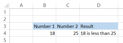
To check whether 18 is greater than 25, we will use the formula =IF(B4>C4, TRUE, FALSE) in cell D4. The result that we will get is:

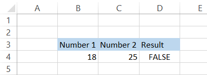
The Excel checks the condition and interprets it as "No, 18 is not greater than 25" and returns the result as FALSE. You can also update the formula to give specific text values in case the condition is fulfilled or not.

By using the combination of CONCATENATE and IF function using the formula =IF(B4>C4, B4&" is greater than "&C4, B4&" is less than "&C4), you can also make the formula dynamic.

With the numbers 18 and 25, the new formula will give you the result:

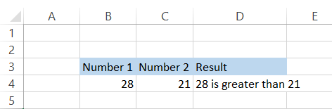
Now try changing the numbers to, let's say, 28 and 21. You will automatically get the result in cell D4 is:

VLOOKUP()

VLOOKUP(Vertical Lookup) is definitely one of the top five functions in Excel that you must know. VLOOKUP works like picking up apples from the ground that fall from the tree. If the apple is rotten(the value does not match), it will get ignored.

If the apple is fresh(value matches), the result gets displayed. Now picking up 2 or 3 apples from the ground is ok. However, would you pick 1000 such apples as well?

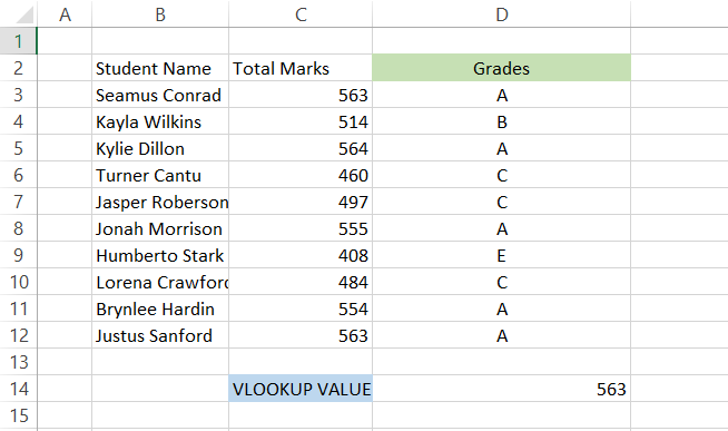
This is where VLOOKUP comes in(now forget about the apples). VLOOKUP will check for a number in the most left-sided column, and if the value matches, it will let us return another value from any column that we state in the formula.

For example, by using the formula =VLOOKUP("Seamus Conrad," B2:D12,2, FALSE), we can return the total marks scored by Seamus Conrad, which are in column two from the left-most column.

If you are still unclear on how to use the VLOOKUP formula, we have an entire article dedicated to it! Check it out here.

HLOOKUP()

If VLOOKUP works on vertically oriented tables, there is just something needed for horizontally oriented tables. This is achieved with the help of the HLOOKUP function that will return a value from a particular row in case the lookup value matches the one on the top row.

Assume that you have the data as illustrated below

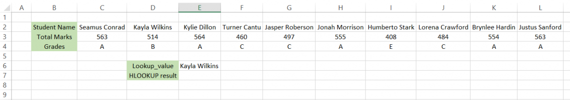
The formula you will use in cell E7 is =HLOOKUP(E6, B2:L4,3, FALSE). Here we have stated row_num from which we want to return the value as three while a FALSE argument returns an exact match for the value. The final result that we get is:

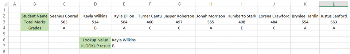
Though it's not necessary that you will encounter horizontal tables on a daily basis, it is quite an important tool if used properly.

We know that the formula syntax can be a bit difficult to understand, which is why we recommend you to read our dedicated article on HLOOKUP, which goes from absolute basics to advance on using the formula.

And if you intend to become a fully-fledged Excel wizard, check out our Excel Modeling Course here!

COUNTIF

The COUNTIF function checks a range of cells for specific criteria and returns the count of the total number of cells that meet the given criteria. Assume that you need to count the number of cells which have numerical values greater than zero.

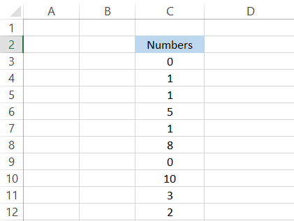
The formula that you will use is =COUNTIF(C3:C12,">0"). This will return the result as eight, meaning eight different cells have values greater than zero. The condition must be specified within the quotation marks; else, Excel will not be able to recognize the argument. 

In this article, we saw some of the most basic formulas you can use in Excel, such as LENS, CONCATENATE, VLOOKUP, HLOOKUP, COUNT, MODULUS, AVERAGE, etc.

However, don't ever underestimate them! They will form the building blocks for most of the complex nested formulas that you might use in real-life scenarios.

If you understand the basic Excel formulas well, you will become an Excel wizard in no time!

Free Resources

To continue learning and advancing your career, check out these additional helpful WSO resources:

• Alphabetize in Excel
• Developer Tab
• Excel Solver
• Index Match Formula
• VLOOKUP