Excel Solver
An optimization tool used to determine the desired outcome by changing a model's assumptions


What Is Excel Solver?
Excel Solver is an add-in optimization tool that is used to find the desired outcome based on changing assumptions of the model. This tool helps those solving complex optimization problems where variables, constraints, and desired outcomes interplay.
Consider scenarios like determining the best combination of stock investments, optimizing resource allocation in a project, or even finding the most cost-effective material mix in manufacturing.
Excel Solver can find the minimum or maximum value in a cell by changing the values in another cell, ultimately leading to the “best” outcome for the problem. It is generally used for simulating different business and engineering models using what-if analysis.
- Excel Solver is an optimization tool used to find outcomes by adjusting model assumptions. It's ideal for complex optimization problems involving variables, constraints, and desired results.
- To use Excel Solver, enable the add-in through Excel options. It helps analyze scenarios and optimize solutions for various problems.
- Excel Solver requires defining objective cells, variable cells, and constraints. It calculates maximum or minimum values in the objective cell by adjusting variables while adhering to constraints.
- The Excel Solver Methods are: GRG Nonlinear, Simplex LP, and Evolutionary are three Solver methods. Each suits different problem types, like linear and nonlinear equations.
- Solver is employed for various applications, from financial planning and resource allocation to pricing strategies and finding optimal production levels. It's especially useful for maximizing profit or minimizing cost in business scenarios.
Enabling the Excel Solver Add-in
The Solver Add-in is generally installed in Excel by default. However, you need to enable it to use it by following the steps below:
- Open the Start menu and click on the Excel icon, followed by double-clicking on the Blank workbook option to create a blank workbook.

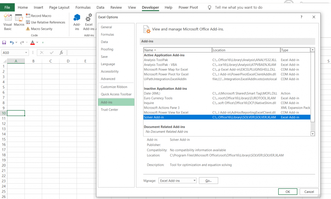
- Click on File and then on Options to navigate yourself to the Add-Ins tab. You will find the Solver Add-in placed within the Inactive Application Add-ins column. First, click on Solver Add-In and then on Go.
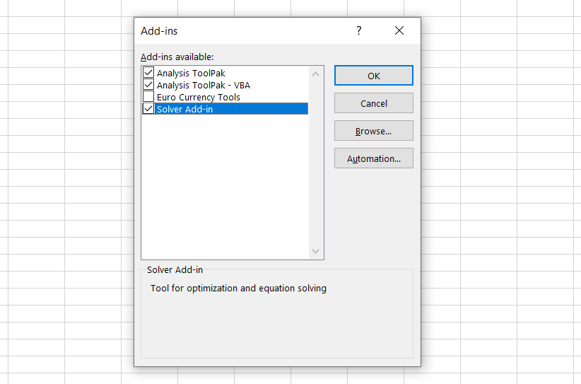
- This will open a new dialog box. Just check the box for Solver Add-Ins and press on OK.
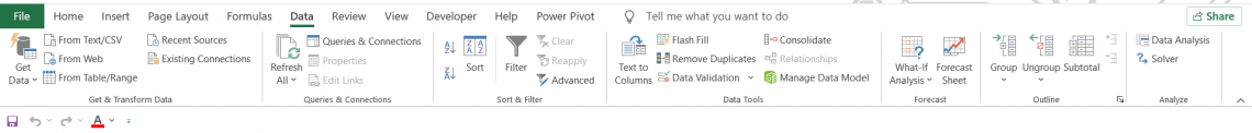
- Now go to the Data tab, where you will find the Solver in Analyze section.
Components of Solver Parameters
The tool requires three different parameters which are set up to find the solution for the problem:
- Objective cell: It represents the goal or objective of our problem. It contains a formula, and it is used to calculate a maximum, minimum, or target value.
- Variable cell: They contain the adjustable data used to obtain the objective cell value.
- Constraints: These are the limitations set up to restrict the solutions from deviating from objective value. Simply put, constraints are the conditions that must be met to obtain objective cell value.
The Solver Parameters window looks as below:

Different types of Solver methods
There exist three different types of Solver methods:
- GRG Nonlinear: GRG is an acronym for “Generalized Reduced Gradient.” This method examines the slope of the objective functions as the input values change to find the optimum solution.
It is fast, but the downside is that it is highly dependent on the initial conditions, meaning that the optimum value will be near the initial conditions laid out. Nevertheless, it is the most used method to solve nonlinear problems. - Simplex LP: LP stands for “linear programming.” The Simplex LP method is used to solve linear problems where the value of one entity is proportional to another entity.
- Evolutionary: The Evolutionary algorithm is slower than the GRG Nonlinear algorithm when used for nonlinear relationships. However, it is more robust and finds a globally optimum solution. Like the theory of natural selection, it weeds out the input values that are not close to the target values to finally reach a stage where the solution represents the closest relation to the target value.
Linear Solutions
Linear equations are the ones that can be solved using methods to find linear solutions. Common examples of linear solutions are age, force and pressure, wages, and hourly rate problems.
The parent and child age difference for different instances of time and their calculation of present age is an example of a linear problem.
You can solve such linear equations in Excel by using the Simplex LP method of Solver. As a result, its application is limited compared to GRG Nonlinear and Evolutionary methods because it cannot be used for nonlinear equations.
However, the solutions obtained by the Simplex LP method are always globally optimum solutions making it a robust method.
Nonlinear Solutions
Solver works best in situations in which nonlinear relationships exist. But, what exactly are nonlinear relationships? A nonlinear relationship exists between two entities when the change in the value of one entity does not correlate with the change in the value of another entity.
On the contrary, linear relationships exist when two entities are proportional to each other.
Linear equations can’t solve nonlinear problems. The most common example is the traveling salesman problem (TSP).

The TSP is a nonlinear optimization problem. It answers how to visit n cities in the fewest possible trips, where each city has an associated cost. Because these problems are easy to describe yet challenging to solve practically, they have garnered people’s attention.
The solutions to such problems are not easy and become more complex if more destinations are added while calculating the best route in these nonlinear optimization problems.

One way to solve this problem is by using Solver methods GRG Nonlinear or Evolutionary methods.
To find an optimal solution for the TSP, one must first create a model with two columns: one for all possible trips and another for total costs. Then, Solver will then assign values for different trip distances and expenses until it finds an answer that satisfies both columns in the model at once.

Case Study for Excel Solver - LP Simplex Method
Excel solver can be used to work on different financial planning tasks, for example, monthly mortgage payments, savings for retirement and business problems.
The calculations behind these complex tasks are elaborate and time-consuming. The tool helps to make such calculations easier based on the availability of inputs from the user.
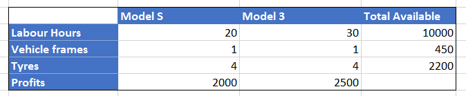
Let’s consider an example of Tesla and its two car models - Model S and Model 3. It requires 20 hours of labor per unit to make Model S, while 30 hours per unit of Model 3.
At the start of the fiscal year, Tesla must decide how many cars to manufacture, given the limited resources. Let’s say it has only 10,000 hours of labor, 300 vehicle frames, and 2,200 vehicle tires available.
Tesla can earn a profit of $2,000 on its Model S while generating a profit of $2,500 on the Model 3. Both the cars require one vehicle frame and four tires on top of the labor hours for making the cars.
Considering the above assumptions, Tesla must decide how many vehicles they will need to produce in the fiscal year to maximize their profit.
The first step is to build a mathematical representation of the business problem and portray it on the spreadsheet.
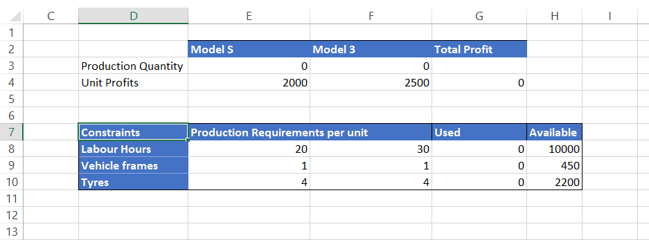
We must determine the values in cells E3 and F3, which are the variables in finding the maximum profit using the available resources. Cell G4 contains the formula =(E4*E3) + (F4*F3) that will calculate the maximum profit Tesla can earn.
Cells E8:E10 and F8:F10 are the production requirements per unit for respective models of Tesla. To compute the total individual resources that will be used to manufacture the cars, we have used the below formulas in cells G8:G10:
G8 = (E8*E3) + (F8*F3)
G9 = (E9*E3) + (F9*F3)
G10 = (E10*E3) + (F10*F3)
These formulas will be used to compare with the available resources to avoid Tesla from overusing its resources.
Speaking in excel terms, cells G8:G10 will represent the left-hand side of the constraint functions, while cells H8:H10 will form the right-hand side of the constraint function in the Solver tool.
Since the spreadsheet model is implemented, let’s move to the Solver to find the optimum solution for our business problem. To run it, just click on the Data in Menu tab, where you will find it in the Analyze section. You can also use the excel shortcut key Alt + A + Y3.
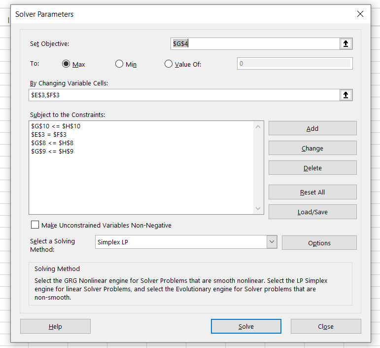
We need to define different components in the parameters window. The first key component to be outlined is the objective cell, whose value can be maximum or minimum or a specific value. The second component is the variable cells.
Based on the changes in the variable cell values, the value in the objective cell reciprocates. The third component is the limitations of the model called constraints. It means that we want our excel model to stick to these limitations, making them a barrier for our calculations.
For example, for manufacturing both car models, we have 10,000 hours of labor available. Hence, one of the constraints can be set up as labor hours should not exceed 10,000.
Similarly, we have set up a few more constraints such as vehicle frames <= 450, tires <= 2,200, and the number of Model S will equal the number of Model 3 in the fiscal year as per the requirement.
Once all the parameters are set up, select the solving method as Simplex LP. Then, make sure you tick the box that says, ‘Make Unconstrained Variables Non-Negative’ and click on Solve.
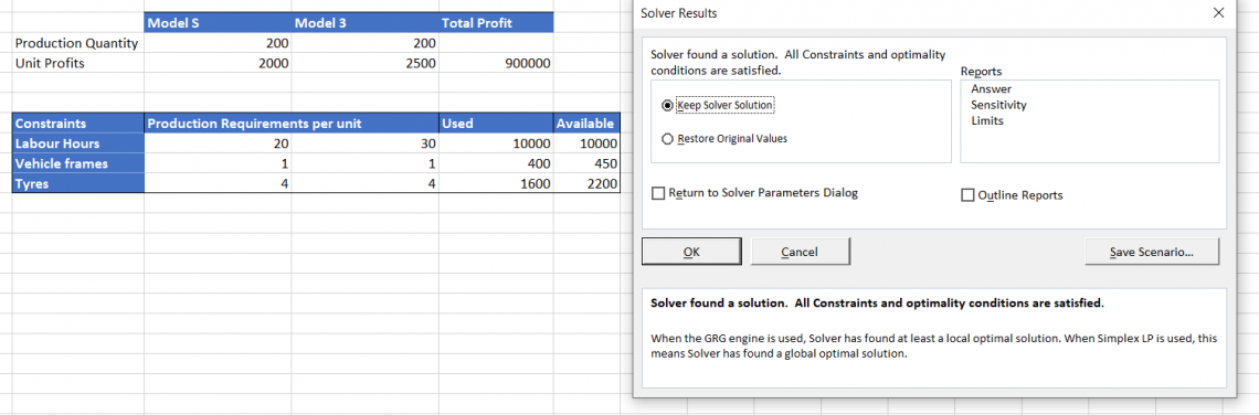
A dialog box should pop up that says, ‘Solver has found a solution.’ This means that Excel has given us the output adhering to all our constraints. From this, we can determine that Tesla can produce 200 cars each of Model S and Model 3 while consuming 10,000 hours of labor work completely.
The other resources, i.e., Vehicle frames and tires, are in excess and are to be stored in inventory.
Case Study for Excel Solver – GRG Nonlinear Method
Let’s formulate the model upon which we need to run our Solver in the spreadsheet. In this hypothetical example, we will try to find the solution for a simple nonlinear problem
Suppose that we (Wall Street Oasis) intend to introduce a new course called ‘Credit Analyst’ in the market. For this, we need to invest $5,000 (no, not our actual cost but a nominal figure for this example), which represents the expenses towards the investment experts team and other miscellaneous costs.
We need to estimate the selling price of the course that helps us recover our investment in one year.
Our spreadsheet model for the problem is as below:
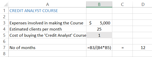
Now let’s run the Solver tool to find the solution for our problem. Use the keyboard shortcuts Alt + A + Y3 to open the solver parameter window. Our Objective cell will be the one that contains the formula, which is cell B7 here.
Since we know the number of months to pay for expenses, we will select the ‘Value of’ radio button and set the value as 12.
Our variables are estimated clients per month and buying costs that we will set up for our course, based on the fact that the number of clients each month won’t be constant.
We have also set up our constraints which we do not intend to cross, i.e., in this case, the course price of $5,000 and unique clients each month (base case scenario), which are <= 15.
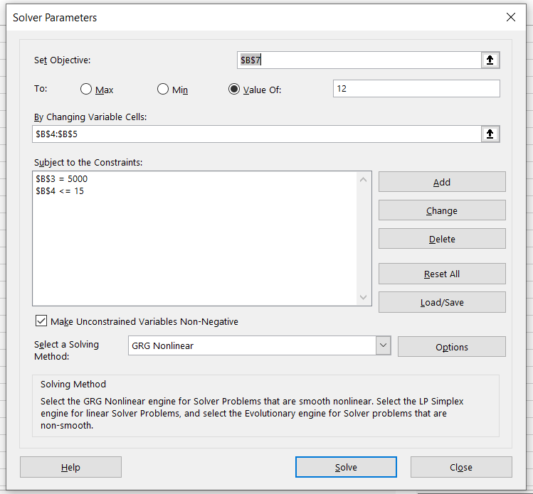
Once all the parameters are set up, select the solving method as GRG Nonlinear method. You will get the solution for the problem as below:
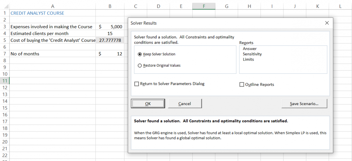
As you can see, the tool satisfies all the conditions and gives us a selling price on the ‘Credit Analyst’ course of approximately $27. (That is the actual price of most of the mini-courses! Check them out here!)
All the assumptions made are modeled upon base case scenarios and can be tweaked to find the best- and worst-case scenarios.
Note
Always remember to avoid keeping your variable cells empty. In this case, we had assigned the value of $1 to cell B5 to avoid getting an error while using the Solver.

Case Study for Excel Solver – Evolutionary Method
Let’s assume that a movie theater showcases six different movies.
The customers can watch a single movie (check the image below for individual prices) or buy the entire bundle at $48.50 and $60.70 for teenagers and adults, respectively. So, of course, the movie theater owner wants to find the optimum price of the bundle and individual movies to maximize their profit.
We have created the spreadsheet model based on the data below:
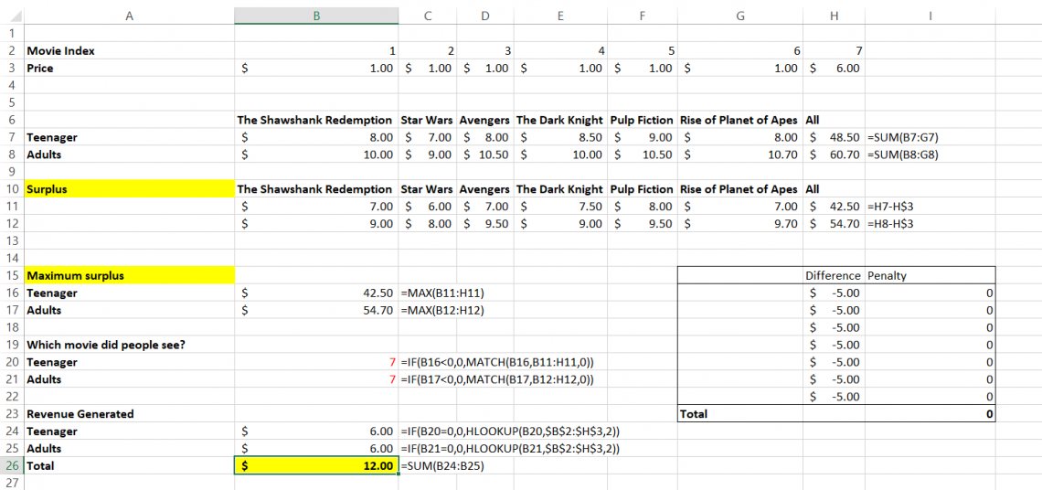
A bit complicated? Maybe, but we will make it easier for you to understand. Our objective cell is B26, while our variables are in range B3:H3. Range B7:H7 shows us how much it will cost teenagers to watch individual movies and buy the entire bundle ($48.5).
Range B8:H8 gives the pricing guide for adults to purchase a ticket at the movie theater and the purchase price of the whole bundle, which is $60.70.
Next, we determine how much surplus is charged for the individual movies and the entire bundle. Here we have subtracted the ticket prices by our variable range B3:H3.
Next, we find the max from ranges B11:H11 and B12:H12, respectively. This portrays our maximum surplus price from each movie and bundle.
See that penalty table in our spreadsheet? It is an additional constraint check that will lower our maximum revenue if the individual price of the movies is greater than the entire bundle.
The final step is to find the revenue generated from both age categories to achieve maximum profit with optimum prices. We have set up our constraints as below:
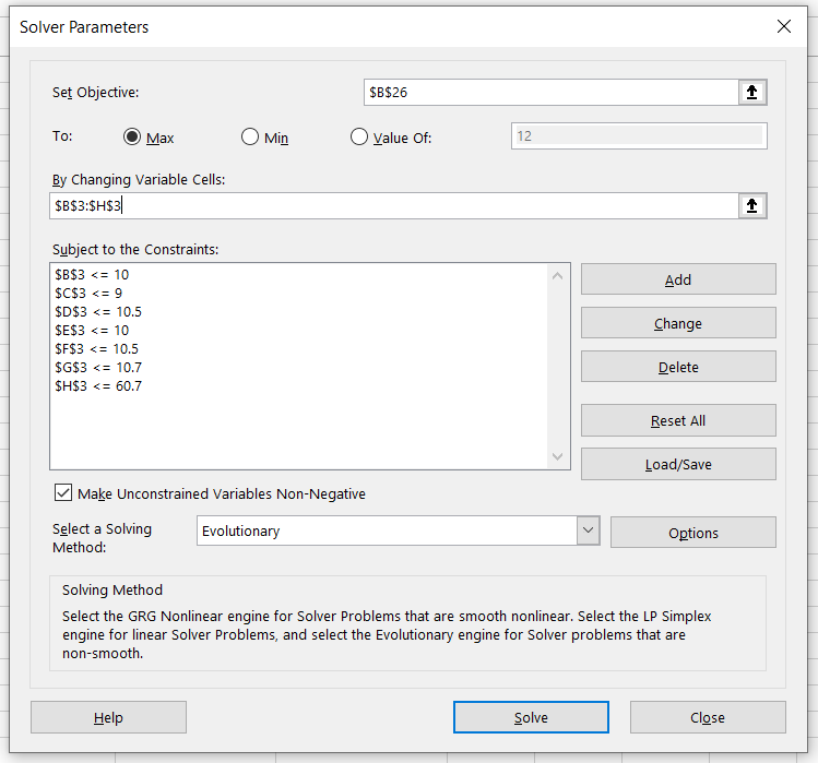
The constraints set up are such that the maximum price of the individual movies or the bundle should not exceed the complete pricing guide for teenagers & adults while buying the movie ticket.
Now select the Evolutionary method of solving and click on Solve. The Solver gives the following result:
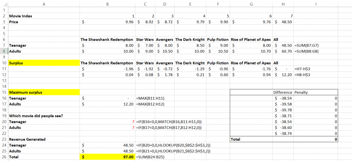
Thus, the movie theatre owner can generate maximum revenue of $97.00, while the optimum prices for the individual movie tickets are in cell B3:H3.
Multi-objective and Mixed-integer Nonlinear Problems
A typical Solver problem has a single objective: to minimize or maximize a target cell. However, many modeling applications require multi-objective and mixed-integer nonlinear problems.
A multi-objective optimization problem has two or more objectives, and a mixed-integer nonlinear programming problem combines two types of constraints: linear and nonlinear.
To determine how to solve a multi-objective or mixed-integer nonlinear problem using Excel 2010, you can use the Gurobi Optimizer add-in that will identify the optimal solution based on your specific model.
Next, we’ll explore how to implement the Solver tool for solving multi-objective and mixed-integer nonlinear problems in Excel 2019.
Solution for Multi-Objective Nonlinear Problem
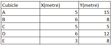
Let’s assume that a company needs to install a coffee vending machine on its first floor consisting of five cubicles. The coordinates for the cubicles are as below:
The first objective is to minimize the distance of vending machines from each cubicle, while the second objective is to install the vending machines as far as possible from the washroom on the same floor.
The coordinates of the washroom are given in the cell L11:M11 (x = 6, y = 14), while our variable cells are L7:M7. These variables will determine where the coffee vending machine must be set up so it’s close to each cubicle.
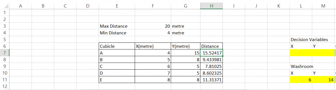
Next, we find the distance between the cubicles and the variables in L7:M7. This will be calculated in the range H7:H11 by using the formula =SQRT(($L$7 - F7)^2 + ($M$7 - G7)^2) in cell H7 and dragged up to cell H11.
Since the distance between the vending and the cubicles is calculated, we need the total length for all cubicles to vending machines by using the formula =SUM(H7:H11) in cell N7.
This is our first objective function, while cell N11 gives our second objective function that consists of the formula =SQRT((L7 - L11)^2 + (M7 - M11)^2). This is the distance between the coffee vending machine and the washroom.
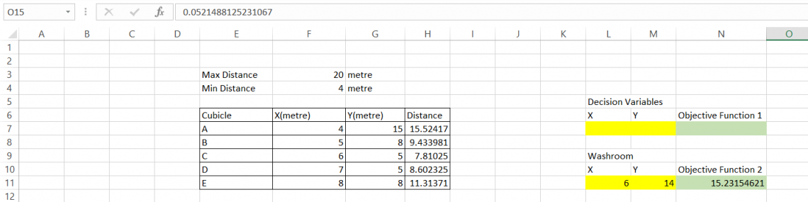
Now we determine the minimum distance of vending machines from each cubicle in cell O14 by using the formula =N7/N11.
Next, we calculate the maximum distance between the vending machine and the washroom in cell O15 using the formula =N11/N7. First, we use the Solver with the O14 cell as the objective value.
Our variable cells will be L7:M7. Our constraints will be H7:H11 <= 20 and H7:H11 >= 4 as given in the data.
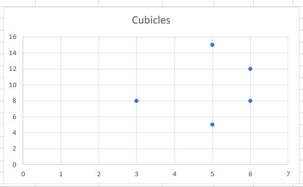
When we run Solver, the distance obtained for goal 1 is 2.80m, for which the coordinates are x = 5, y = 1.
Similarly, when O15 cell is the objective value, with similar variables and constraints, the distance obtained is 0.05m, for which the coordinates are x = 7.8 and y = 13.8.
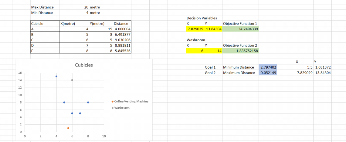
The scatter plot for the two goals is given below:
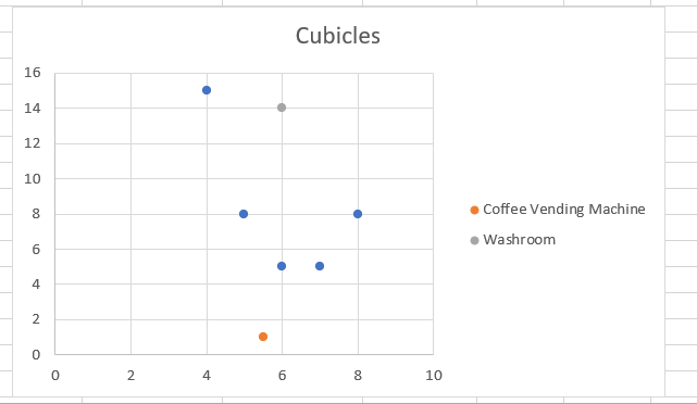
In this way, a multi-objective nonlinear problem can be solved. Furthermore, optimum solutions can be solved by adding more constraints to the situation to get a “good” answer.
When to Use Excel Solver?
Excel Solver is a tool that can find the desired outcome by changing assumptions in a model. The program has many uses and is often used for business, engineering, and science applications.
For instance, it can find optimal production levels and product pricing decisions for a company. It can also help customers determine the best payment plan by calculating various loan payments and down-payment alternatives.
Solving problems with Solver is particularly relevant for businesses or organizations that need to maximize profit or minimize cost. This type of software relies on mathematical equations to find the solution.
However, it may not be appropriate for all kinds of problems because it assumes no constraints other than the ones given in the problem description.
Free Resources
To continue your journey towards becoming an Excel wizard, check out these additional helpful WSO resources.


or Want to Sign up with your social account?