IFERROR Function
It returns a customized result whenever it evaluates and catches an error.


What is the IFERROR Function?
An IFERROR function returns an alternative result, usually text, instead of returning an error if one would have been replaced. By acting as a trap for catching errors, the function ensures efficient handling of errors from formulas and functions in Excel.
Generally, when you input a formula in Excel, it makes calculations in the background and returns the result to the user.
However, sometimes, you can get an error value in the cell. As a result, you may have to manually assess the formula's incorrect and edit the procedure accordingly. Once corrected, Excel will return the correct calculation in the spreadsheet.
We need to catch those errors since they do not collaborate with the rest of the data efficiently and can bring inaccuracy in the results that Excel returns.
Sometimes, going through all the errors and reassessing them might not be very important. That is where this logical function comes in.
This article will guide you on how you can catch different errors by using just the ultimate error-management function. It takes care of all error types: #N/A, #VALUE!, #REF!, #DIV/0, #NUM!, #NAME?, and even #NULL!
Key Takeaways
- An IFERROR will catch all types of errors: #N/A, #DIV/0!, #NULL!, #NAME?, #REF!, #VALUE!, and #NUM!
- If the value_if_error argument is an empty string (“”), Excel returns the result as an empty cell if an error is identified.
- The value argument will be considered an empty string (“”) if it is blank, rather than an error.
- You can use a combination of IF and ISERROR for all versions of Excel before 2007 for error management. Subsequent versions have this function built in.
- Value_if_error can be a custom text string, empty string, number, formula, boolean value, or the result of a formula, depending on the referenced cell or hard-coded value.
Understanding IFERROR function
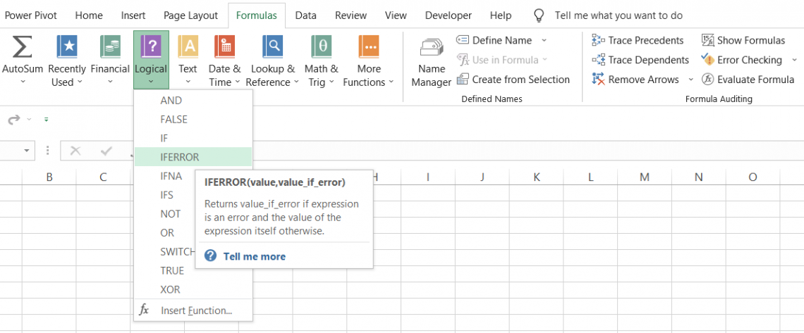
The function is categorized as a Logical function. Therefore, it returns a customized result whenever it evaluates and catches an error.
If we break down the formula, we see that the function combines two traditional Excel functions - IF and ISERROR. Both logical operations can evaluate if the cell or procedure consists of an error.
But Microsoft had something else in mind. They came out with a dedicated function besides our IFERROR function.
The function works in two simple steps:
- Search a cell, reference, or formula for an error.
- If the outcome of the condition is TRUE, return the desired result.
When writing complex formulas, it is pretty common to face different errors. Some functions, such as VLOOKUP, HLOOKUP, and INDEX-MATCH, give errors that need to be handled to avoid messy spreadsheets.
Excel has a solution to all of our problems in the form of just one simple function.
Understanding the types of errors in Excel
We have the ultimate tool to combat errors, but it is equally essential to understand the different types of mistakes you might encounter while working in Excel. They are:
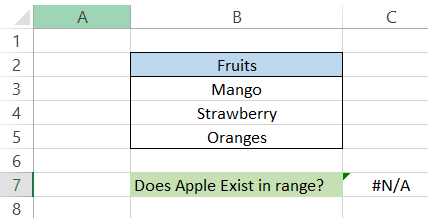
1. #N/A - This error occurs when Excel cannot find a value in a referenced range of cells.
Suppose you use VLOOKUP to find 'Apple' among a range of fruits: Mango, Strawberry, and Oranges. Excel will return the #N/A (not applicable) error.
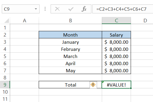
2. #VALUE! - Excel returns a #VALUE! Error when the values provided in the formula are of an unsupported type or, in general, when there is something wrong with the way the procedure is typed.
For example, as we unintentionally referenced the text in cell C2 for our total sum, Excel has returned a #VALUE! Error.
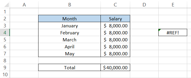
3. #REF! - These errors occur when you reference a particular cell or range of cells in the function that become invalid due to the row/column getting deleted or when the formula gets copied to a new position where the reference becomes null.
For example, we referenced five cells in our SUM formula in cell C9. If you copy the formula to the cell less than five cells above the target cell, you will get the #REF! Error( cell E4).
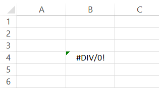
4. #DIV/0! - When you divide a number by zero, you will get a #DIV/0 error. For example, try dividing 101 by 0 in Excel, and you will get the result #DIV/0.
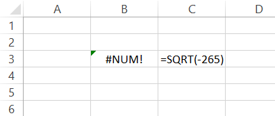
5. #NUM! - These errors usually occur when a number is too big or small, making it impossible to perform numerical calculations due to an invalid numeric value.
For example, if you try to take the square root of a negative number in Excel, you will get the #NUM! Error.
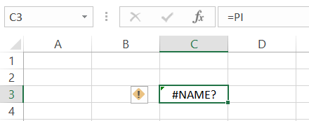
6. #NAME? - The #NAME? An error occurs when quotation marks are missing around a text string in the formula, a function name is misspelled, or Excel doesn't recognize something. Something needs to be corrected in the recipe.
For example, if you are using the PI function in Excel and forget to use parentheses, you will get the #NAME. Error.
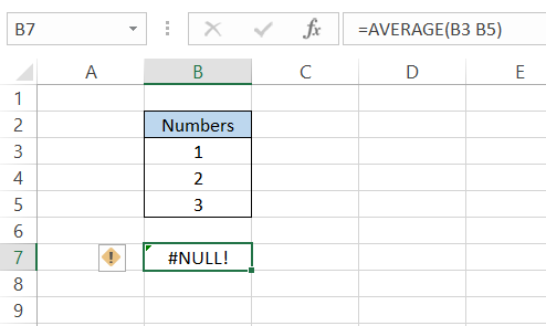
7. #NULL! - When a range of cells is incorrectly referenced or if you forget to use range operators such as colon (:) or comma (,) in the formula, Excel will return the exceptionally rare #NULL! Error.
For example, if you find the average of the first 3 numbers using the AVERAGE function and forget to add a colon (:) between the starting and ending cell range, you will get the #NULL! Error.
Syntax and example of IFERROR Function
The syntax for the function is
=IFERROR(value,value_if_error)
where,
value = (required) A value, expression, cell reference, or formula must be checked for an error.
value_if_error = (required) The value that needs to be returned if an error is found. It can be a customized text string, an empty string (blank cell), a number, or another formula.
It is important to remember, while using the function, that it will mask all types of errors in the spreadsheet. Some errors need special attention, such as reference errors, where cell values are connected to different workbook parts.
Apart from this drawback, the function does an excellent job of tackling all the types of errors in Excel.
Example:
The simplest example you can use to understand how the function works is the division of one by zero in Excel. Our data is illustrated below:
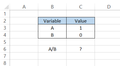
Suppose that we decide to return the text string "The formula has returned an error!" if Excel returns an error. We will use the formula =IFERROR((C3/C4), "The formula has returned an error!"), returning the following:
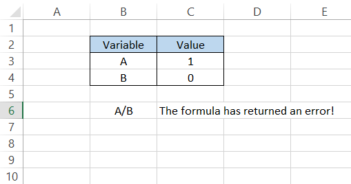
As 1/0 gives us the #DIV/0 error, and IFERROR is adept at catching those miscalculations, we get a customized text string as our alternative result.

IFERROR along with lookup functions
The most common error you will encounter while using lookup functions, VLOOKUP, HLOOKUP, INDEX-MATCH, or even XLOOKUP, is the #N/A error.
When you reference a range of cells in a formula, and VLOOKUP cannot find the lookup_value, Excel will return the #N/A error.
Example #1
When you perform a recon task (apples-to-apples comparisons), error feedback about values missing in the referenced range is usually welcomed.
In other instances, you can nest the VLOOKUP inside the IFERROR function to give you a more friendly result (although you should never trap errors without reason).
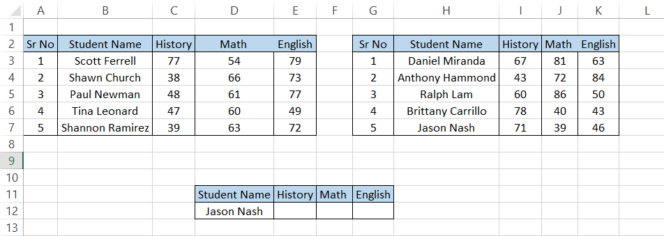
For example, assume that you have data for the marks scored by students, as illustrated below, and need to find what "Jason" scored in his examination.
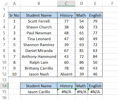
However, you confuse Jason's last name with another student (Brittany Carrillo) and use the VLOOKUP formula as
=VLOOKUP(B15, B2:E12,2, FALSE)
which gives you the #N/A result.
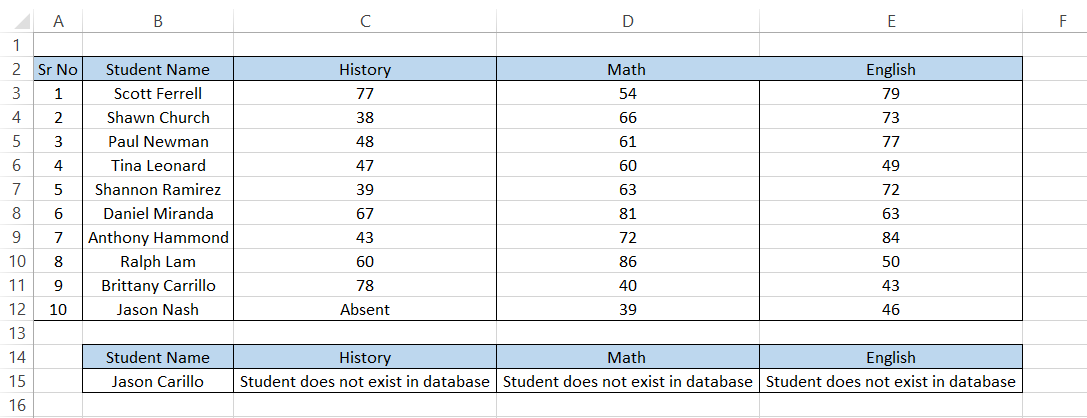
This error can be avoided by using the formula:
=IFERROR(VLOOKUP(B15, B2:E12,2, FALSE)
"Student does not exist in database"), which will give you the result:
The INDEX-MATCH combined function can also return an #N/A error when the look_up array and return array are of different sizes. In such cases, it is advisable to recheck the referenced ranges before using the function.
Example #2
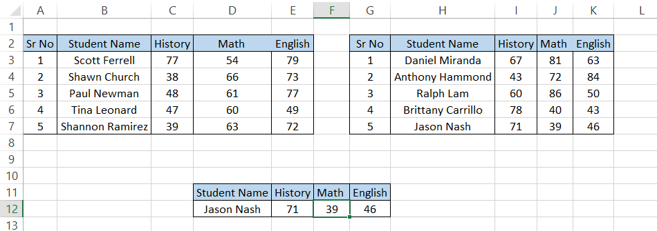
Let's say the teacher has two lists of students from which the score for Jason Nash needs to be determined. The data for the scores are illustrated below:
We know that we can only reference one table in our VLOOKUP function. Even if we reference the entire dataset, our lookup_ranges exist in different columns. Here, you can use a combination of both functions.
You know that if the value does not exist in the lookup_array, we will get an #N/A error. So, based on this principle, we will nest another VLOOKUP function inside the formula that has our second table as the lookup_range.
The formula that you will use in the spreadsheet is
=IFERROR(VLOOKUP(D12, B2:E7,2, FALSE), VLOOKUP(D12, H2:K7,2, FALSE))
which will give you the result:
We have always stressed how you can do the same thing differently in Excel.
You guessed right if you have already read our articles on IF and IFS statements!
You can use nested IF/IFERROR/IFS statements to give you the same result in Excel. When you start being creative in spreadsheets, the sky's the limit!
Why use IFERROR cautiously
When preparing complex financial models, there is a high probability that you will face different types of errors, such as #REF! or #DIV/0! Therefore, the most logical step is to address those errors individually rather than using the function.
For example, let's say that you need to address a #DIV/0 error that results from dividing a number by zero.
If you think," Alright, I don't have time to play around! I will return "Error!" for all the #DIV/0 errors using the error-management functions in Excel"; that is the wrong approach.
Suppose you use the VLOOKUP formula and Excel cannot find the referenced cell. This will result in a #REF! Error in the spreadsheet.
The cause for the error cannot be recognized unless you analyze the formula. Perhaps, while deleting extra rows or columns, the reference for the recipe changed, giving you the error.
So this means that always using this type of logical function is not feasible. Make sure that you evaluate the type of error returned below using the function, as it becomes quite difficult to keep track of all the errors if ignored or addressed using a single function.
Other error-management functions
Handling different types of errors using the same IFERROR function can be risky while preparing Excel models. Excel provides you with different behavior-specific alternatives that you can use for error management, such as:
1. ISERR function
ISERR evaluates and returns TRUE for all error types in Excel except for #N/A. For example, if you have different errors in spreadsheets and use the ISERR function, you will get the result as illustrated below:
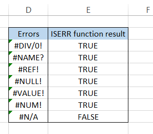
As you can see, by using the =ISERR(D3) in cell E3, the function returns TRUE for all the errors except #N/A. You can use a combination of IF and ISERR to return the desired value based on the error received, i.e., #N/A or anything else.
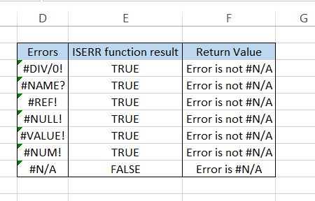
We have used the formula =IF(ISERR(D3), "Error is not #N/A," "Error is #N/A"), which, if evaluates as TRUE, will return the value, "Error is not #N/A," or "Error is #N/A" for FALSE.
2. ISERROR function
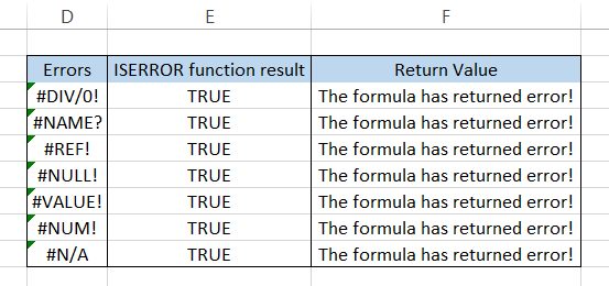
The ISERROR function will evaluate and return TRUE for all error types in Excel. The combination of ISERROR and IF can be used as an alternative to the function since both methods can get the same result in a spreadsheet.
For example, we can use the formula =IF(ISERROR(D3), "The formula has returned an error!", "Not an error"). Then, whenever Excel encounters an error, ISERROR and IF will evaluate as accurate, returning "The formula has returned an error!".
On the other hand, when they evaluate it as false, it returns "Not an error."
3. ISNA function
While ISERR returns TRUE for all error types except #N/A, the ISNA function works in precisely the opposite manner.
The ISNA function will return true only for #N/A errors, while all the other errors will return as FALSE. So, for example, when you use the formula =ISNA(D3) for different errors, you will get the result as FALSE, except for #N/A.
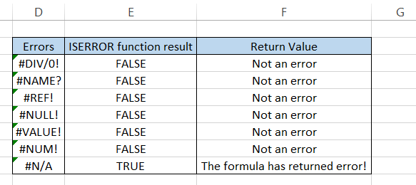
By combining the IF function with ISNA, =IF(ISNA(D3), "The formula has returned an error!", "Not an error"), you can return the desired value in case the ISNA function catches the #N/A error.
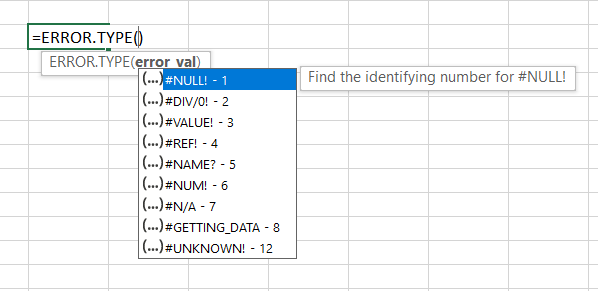
4. ERROR.TYPE
When you use the ERROR, TYPE function in Excel, it returns the number that correlates to the type of error value you might get while working on a spreadsheet.
For example, suppose you have the #NULL! Error in Excel and use the formula =ERROR.TYPE(C3). It will return 1.
Based on the ERROR.TYPE result, you can use nested IF or IFS statements. This will make it such that if a cell has a #DIV/0! Error, for example, you will get one result and another completely different result for a #NAME? Error.
One important thing to note about ERROR. The TYPE function is that if Excel can find none of the errors in the referenced cell, then the formula will return an #N/A error.
5. IFNA function
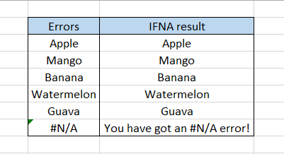
If you don't feel like using a combination of the ISNA and IF functions to return different values for TRUE or FALSE on error evaluation, you can use the IFNA function that works similarly.
For example, the formula =IFNA(D3, "You have got an error!") will give you the following result:


or Want to Sign up with your social account?