Excel for Beginners
A “Dummies” Guide for Beginners


excel Fundamentals
These are some of the fundamental elements of Excel that you should become familiar with before you start working with functions and values.
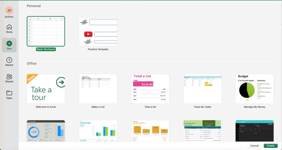
1. Opening a Workbook
When you open Excel, you will encounter this screen. From here, you can
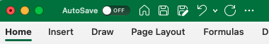
2. Understanding the Ribbon
The ribbon is the area where the majority of the functions of Excel are. This is where you change fonts, insert graphs, find mathematical operations, and much more. Being familiar with the ribbon is essential to becoming more efficient, so experiment with it a bit.
Most of the time, you will be on the Home tab, but the Formulas and Data tabs are also helpful.

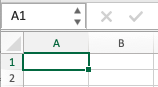
3. Understanding the Formula Bar
The formula bar is directly below the ribbon, and will see the values and functions you have plugged into a specific cell. You can see which cell you are currently in by looking at the far left side of the formula bar. In this case, we are presently in cell A1.
Also, by clicking on ƒx, you can browse all the formulas available.
![]()
4. Customizing the Quick Access Toolbar
The quick access toolbar is in the top left of your spreadsheet (the green bar). The default toolbar includes:
To customize the functions in this toolbar, click on the three dots on the far right of the quick access toolbar.
5. Saving and Sharing Workbooks
To save or share a workbook, go to File on your screen. From here, you can save your workbook as a file or a template. Templates can be used later to save time because you already have formatted some worksheets.
For example, if you had a budget table but needed to do a new one every year, you could have the skeleton of the table and input the new values into the template each year.
6. Workbooks vs. Spreadsheets
A workbook is an Excel file that includes all of the spreadsheets. A spreadsheet is an individual sheet in the workbook.
These different spreadsheets are accessed at the bottom, with each tab (spreadsheet) being labeled differently. The default workbook starts with only one spreadsheet.
To add a spreadsheet to a new workbook, click on the plus sign next to "Sheet 1" on the bottom. Each sheet can be renamed by double-clicking on the name.
Key Takeaways
- Excel works like a database with cells containing values, dates, names, and functions. It is a powerful tool for performing complex calculations and organizing large datasets.
- It is widely used in industries such as corporate banking, private equity, investment banking, equity research, investor relations, and corporate development. Learning Excel can give you a competitive advantage in job searching.
- Understanding the Excel interface is crucial for efficiency. Familiarize yourself with elements like the Ribbon, Formula Bar, Quick Access Toolbar, and saving/sharing workbooks.
- Learn how to reference cells, use relative vs. absolute cell references, enter data, and perform basic calculations like addition, subtraction, multiplication, and division.
- Master formatting worksheets for clarity and organization. Familiarize yourself with basic functions like SUM, MIN, MAX, AVERAGE, MEDIAN, COUNT, IF, and AutoSum to perform calculations quickly and accurately.
Excel Basics
Now that we have some of the fundamental aspects of Excel, we can move on to the basics of executing actions.
1. Understanding Cell References
Each little box is called a cell. The cells are organized horizontally by letters (A, B, C) and by numbers (1, 2, 3) vertically. The intersection between the row and column is the cell. For instance, if you want to reference the top left corner cell, it is called A1.
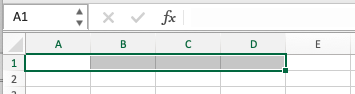
You can also select multiple cells, known as a cell range.
If you want to perform a calculation on a range of cells, let's say from A1, B1, C1, and D1, you could use the notation A1:D1.
When you click on a cell, the cell name will be listed in the left corner of the formula bar.
2. Relative vs Absolute Cell References
There are two different types of cell references when formulas are copied and filled into other cells:
1. Relative cell references count cells from a particular location.
For example, if you reference cell A2 from A4, you are referring to the cell that is up two compartments in the same column.
If you were to copy the formula somewhere else, it would always refer to the cell two cells up in the same column. So, for instance, if you input the formula into cell C7, it would refer to cell C5.
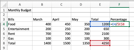
2. Absolute cell references remain the same no matter where the formula is copied. For example, if you always want to reference cell E8, then you would put $E$8.
For instance, let's say you are calculating percentages, and cell E8 has your total.
Percentages are calculated by dividing by the total, so now, no matter what data points you use, you will constantly be dividing by E8 when you use $E$8. The relative location of cell E8 doesn't matter anymore, so the calculation for cell F5 will also divide by cell E8.
Partially locked cell references can also be used, locking the column or row alone. To do this, simply add a dollar sign in front of the coordinate you want to lock (e.g., $E8 to lock the formula on column E).
To quickly cycle through relative/partial/absolute/references, use F4 while your cursor is on the reference.
For more information on the differences and how to use them, you can visit here.
3. Formulas vs Functions
Both of these are methods to perform calculations.
-
Formulas are an expression that requires manual input. For example, if you wanted to add a range of cells, you would say =A1+A2+A3. This is more labour-intensive than functions, which you will see below.
-
Functions, on the other hand, automatically perform the calculation for the range of cells. This is more efficient and eliminates the risk of errors. For example, if you wanted to add those same three cells above, you would say =SUM(A1:A3).
4. Entering Data
You can input values into a cell by either clicking on it or typing it into the formula bar. In addition, you can copy and paste any data from other spreadsheets or sources.
Cells can contain text and numbers. Some examples of this are:
- Currency
- Percentages
- Dates
5. Basic Calculations
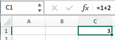
One of the essential tips you need to know: calculations always start with an equals sign (=). So, for example, if you wanted to add two numbers (1+2), you would input =1+2 into the cell.
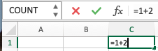
After inputting this calculation, press enters, and your answer will be displayed. You can still observe the formula in the formula bar if you forget what formula or numbers you put in the cell.
Similarly, if you wanted to add values from two different cells, you would insert =B2+B3, for example.
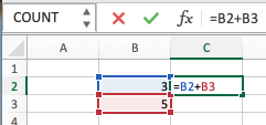
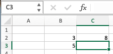
With these cell references, the total will automatically account for that change if you change the number in either B2 or B3.
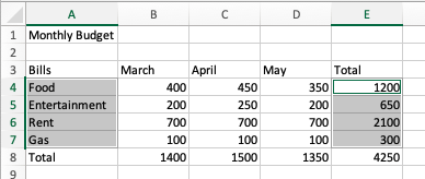
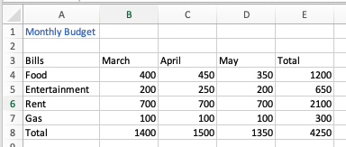
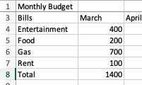
6. Hiding and Unhiding Rows or Columns
You can hide columns or rows if you want to clean up your spreadsheet to make it look more organized without deleting values. You can hide or unhide by clicking on the line while holding Control between two letters or numbers.
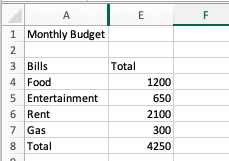
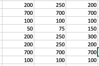
Notice below how columns B, C, and D are now hidden to only show the total values. This makes a cleaner spreadsheet while also keeping the values.
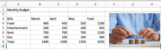
7. Inserting Images
To insert an image, go to the Insert tab in the ribbon. There is a Pictures option that allows you to import a picture from:
- Photo browser
- From files
- Stock images
- Online
8. Creating Charts
Under the same Insert tab as the Pictures option, there are numerous options for charts and graphs:
- Pie charts
- Line graphs
- Scatterplots
- Histograms
- Bar graphs
There is also a Recommended Charts option that gives suggestions based on your highlighted data. For example, you want to highlight the cells with data labels and the values.
For example, if we wanted a pie chart of the totals alone, it would look like this:
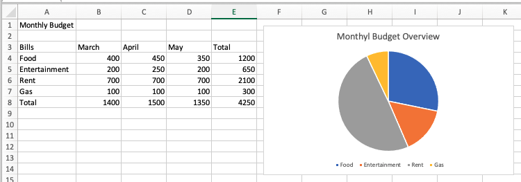
To edit elements of the chart, such as axis labels or the legend, double-click your mouse on the chart, which will show an Add Chart Element button in the ribbon.
9. Understanding Errors
If an error occurs, this icon will show up:

There are many causes of errors, so if you click on the yellow triangle, it will briefly explain the problem. For example:
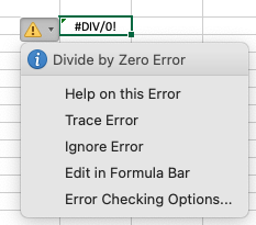
There are a few options to solve the problem. First, if the issue is not imperative, you can choose to ignore the error, and the yellow triangle will disappear.
To find errors in your spreadsheet, go to the Formulas tab in the ribbon and then click on the Error Checking button.
10. Inserting Formulas
Remember that using a formula is the manual way to make basic computations instead of using functions. This can include:
- Addition (A1+A2)
- Subtraction (A1-A2)
- Multiplication (A1*A2)
- Division (A1/A2)
- Exponents (3^2)
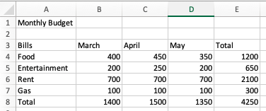
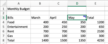
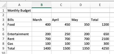
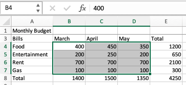
For example, if we wanted to calculate the totals for March, April, and May, we would like to add B8+C8+D8:
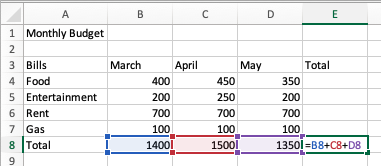
Note that pursuing this method of calculating the total will highlight the cells involved in the calculation. After typing in this equation and pressing enter, we get 4250.
Keeping the order of operations in mind if you are doing multiple computations in a single formula is crucial.
Parentheses → Exponents → Multiplication → Division → Addition → Subtraction
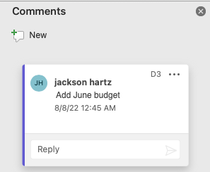
11. Comments
Leaving comments on your spreadsheet can be beneficial for remembering certain things or working on a shared workbook. You can leave a comment by going to the top right of the ribbon.
For instance, let's say I wanted to add the June budget but didn't want to forget; I could add this comment:
Formatting Worksheets in Excel
This section has to do mostly with the appearance of your spreadsheet to ensure it is clear and organized.
1. Font formatting
Fonts can be changed under the Home tab in the ribbon. You can change the size, font type, and color.
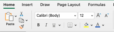
For instance, if I wanted to make "Monthly Budget" blue:
2. Insert New Rows and Columns
You can add cells if you need to input more data in your already-constructed spreadsheet. For example, let's say you want to add a row. You start by clicking on the row number where you want to insert a column.
On a Mac, you would click while holding Shift-Command-Plus Sign; on a PC, you would hold down Control-Shift-Plus Sign. This will always add a column to the left or a row on top.
3. Editing Column Width
Changing the width of the column allows you to read what the cell says when the words are longer than the current cell size allows. For instance, if you look at cell A5, it is supposed to say entertainment, but you can only read "entertainment."
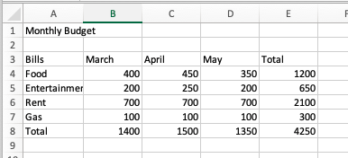
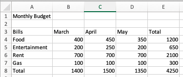
To fix this, click and hold on the line in between columns A and B, then drag right until you can see the whole word, as seen below:
4. Freezing Labels
Let's say you have a spreadsheet with thousands of rows of data. When you're looking at row 2000, you do not want it to look like this, where you can't see the labels:
To fix the labels in place, you can go to the View tab of the ribbon and then to the Freeze Top Row button because that is where the tags are.
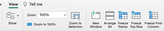
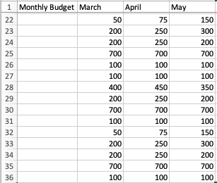
Even though we are further down the spreadsheet, the column labels are still visible.
5. Sort Data
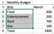
You can sort data by numerous criteria. In this case, we will sort the bills in alphabetical order.
First, highlight the data we want to alphabetize:
Then, under the Data tab of the ribbon, there is a Sort button:

In the window below, we can specify how we want the data. The default shown here is alphabetical, from A to Z, which is what we are looking for.
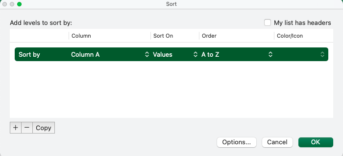
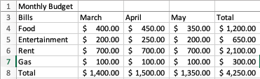
The result of this sorting by alphabetical order is shown below.
6. Formatting Currency, Percentages, Dates, etc
If we want money to show up with the dollar sign ($) or percentages to appear with the percent sign (%), we can change this by going to the Home tab in the ribbon.
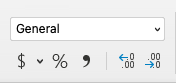
Here, we can change the number values to different currencies or change values to percentages.
Some other number format options are:
7. Understanding the format painter
The format painter can be helpful when you want to use the same formatting for multiple spreadsheet parts. In other words, it copies and pastes a format. The symbol looks like this and can be found under the Home tab in the ribbon.

This can improve efficiency, so you do not have to change the format for everything manually.
8. Conditional formatting
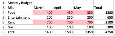
Conditional formatting changes the format based on certain conditions. For example, let's say we wanted values above 250 to be highlighted in red. But first, we need to highlight the cells to which we want the condition to apply.
Next, under the Home tab in the ribbon, there is the Conditional Formatting button:

We go to Highlight Cell Rules and then Greater Than…, which brings up this window:
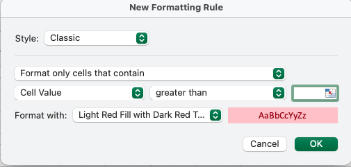
We would then put 250 into the value box to highlight any cells more significant than 250 in a light red fill with dark red text.
Basic Functions of Excel
These are some fundamental and common functions you may use in Excel. To increase efficiency, parts make calculations faster and more accurate than inputting formulas.
You can browse the functions under the Formulas tab in the ribbon. Functions start with the equal sign (=), the position, and then the arguments (the values you put in the part).
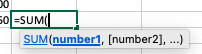
Let's take the SUM function, for example. You can click and highlight multiple cells to perform the function.
You can type it in or click on the formula bar to get the function. After you type in the role, it will list the conditions that must be given to perform the calculation.
The function consists of three parts:
- Equals (=)
- Function name (SUM)
- Arguments (number1, [number2],...)
If you want to apply a function to other cells, you can click and drag the cell with the position by the small box (the fill handle) in the bottom right of the cell.
1. SUM
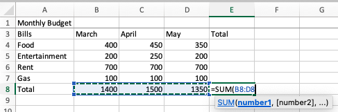
This is the most commonly used function in Excel. Summing is another word for adding. For example, let's say we wanted to add cells B8 through D8 to get the total for the three months:
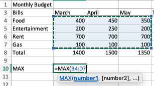
2. MIN and MAX
These two functions find the lowest and highest numerical value in an array. For example, let's say we want to see the maximum bill in our table. Similar to the SUM function, we type the equal sign, then MAX, followed by the cells to get our answer of 700:
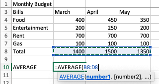
3. AVERAGE
The average is calculated by adding all of the values and then dividing by the number of values. This can be easily done by using the average function. Let's say we wanted to find our average monthly payment:
4. MEDIAN
It is a similar process to finding the average of a function:
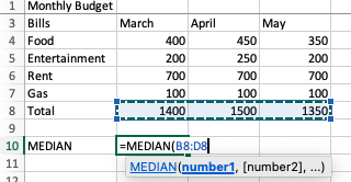
Calculating the median can be helpful as an alternative to the mean if there are outliers in the data.
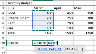
5. COUNT
This function counts how many cells there are that contain numbers. It ignores empty cells and cells with text.
For example, if we wanted to know how many bills we pay each month:
Once we press enter, the answer is 4, which is correct because our four bills are:
6. AutoSum
The AutoSum button makes some of the most common calculations even more accessible. The AutoSum button automates some of the most common functions:
- Sum
- Average
- Count
- Maximum
- Minimum
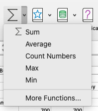
It automatically looks for values above or to the left of the call you are in to choose the range of cells to perform the function on. Make sure that Excel highlights the correct number of cells before you enter to perform the calculation.
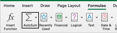
The AutoSum button can be found in the Formulas tab in the ribbon. There are also shortcuts for AutoSum:
| Windows | Shortcut | Mac |
|---|---|---|
| Alt-= | AutoSum | ⌘-Shift-T |
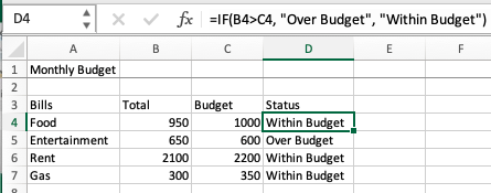
7. IF
These functions are used when you want to sort the data based on specified criteria. The function returns a specific value if it is accurate and a different matter if it is false.
For example, if you wanted to check for values more significant than our budget and display an "Over Budget" message, you could use this function.
This function includes three arguments:
- Condition (B4>C4)
- "If true" value ("Over Budget")
"If false" value ("Within Budget")
There are many other versions of the IF function, such as IFERROR and COUNTIF.
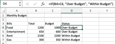
Now, if the total for a bill, such as food, changes, the IF function's status will also change.
Excel Shortcuts
These are some of the most common shortcuts that can save you time and increase efficiency.
| Windows | Shortcut | Mac |
|---|---|---|
| Ctrl-N | Create a new workbook | ⌘-N |
| Ctrl-O | Open a new workbook | ⌘-O |
| Ctrl-S | Save a workbook | ⌘-S |
| Ctrl-Z | Undo the last action | ⌘-Z |
| Ctrl-Y | Redo the last action | ⌘-Y |
| Shift-F2 | Insert/edit a cell comment | ⌘-Shift-F2 |
| Ctrl-Shift-! | Number format | Ctrl-Shift-! |
| Ctrl-Shift-# | Date format | Ctrl-Shift-# |
| Ctrl-Shift-% | Percent format | Ctrl-Shift-% |
| Ctrl-Home | Go to cell A1 | Fn-Ctrl-Left |
| Shift-Spacebar | Select entire row | Shift-Spacebar |
| Ctrl-Spacebar | Select entire column | Ctrl-Spacebar |
| Ctrl-Shift-Arrow | Select to end of the last used cell in the row/column | Ctrl-Shift-Arrow |
| Ctrl-Arrow | Select the last used cell in the row/column | Ctrl-Arrow |
| Ctrl-F2 | Open the print preview window | N/A |
| Ctrl-F1 | Show/hide the ribbon | ⌘-⌥-R |
| Shift-Arrows | Select a cell range | Shift-Arrows |
| Ctrl-Shift-Arrows | Highlight a contiguous range | Ctrl-Shift-Arrows |
| Ctrl-A | Select all | ⌘-A |
| Ctrl-F | Find and replace | ⌘-F |
| Enter | Confirm the change and leave the cell | Enter |
| Esc | Cancel a cell entry and leave the cell | Esc |
| Ctrl-Shift-Left/Right | Highlight contiguous items | Ctrl-Shift-Left/Right |
| Ctrl-PageUp/Down-Arrows | Referencing a cell from another worksheet | Ctrl-Fn-Down/Up-Arrows |
| Ctrl-; | Enter date | Ctrl-; |
| Ctrl-Shift-: | Enter time | Ctrl-Shift-: |
| Alt-= | Autosum | ⌘-T |
| Tab | Accept autocomplete suggestion | Tab |
Although these shortcuts can be complicated to integrate into your workflow initially, once you get them down, it will save you time and minimize the chances of errors.


or Want to Sign up with your social account?