MOD Function
Returns the remainder after a number (dividend) is divided by another number (divisor)


What is the MOD Function?
MOD is an in-built function in Excel that returns a remainder after dividing two numbers, i.e., wherein a dividend (number A) is divided by the divisor (number B). This function falls under the category of Math and Trigonometry functions of Excel.
Suppose you need to calculate the loan amount after every third cell in column D or any other nth value in the entire spreadsheet. MOD plays a critical role in reaching this calculation.
Key Takeaways
-
The MOD function in Excel calculates remainders when dividing numbers. It is categorized under Math and Trigonometry functions and is useful for a variety of tasks related to Excel data manipulation.
-
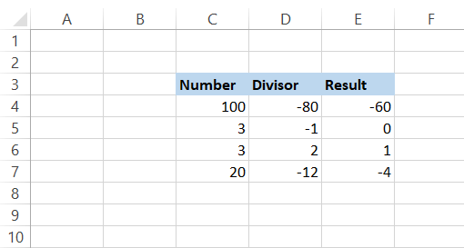
The result of the MOD function takes the sign of the divisor. If the divisor is negative, the remainder will be negative as well, and if the divisor is positive, the remainder will be positive. Dividing by zero results in a #DIV/0! error.
-
The MOD function has practical applications like loan calculations, identifying patterns in rows or columns, executing conditional actions, and combining with other functions for versatile calculations.
Syntax for MOD function in Excel
The syntax for using MOD is as follows:
=MOD(number, divisor)
where,
- number = the dividend or the numerical value we wish to find the remainder. This is a required parameter.
- divisor = the numerical value we divide the dividend in the function. This is a required parameter.
Note
The result of the MOD function will always take the sign of the divisor. So, if your divisor is negative, the remainder will be negative as well. Similarly, if the divisor is positive, the remainder will be positive too. If the divisor is 0, you will get a #DIV/0! Error.
How to use the MOD Function in Excel?
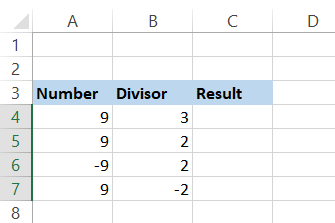
Let’s look at some basic examples of using MOD. The number/dividend in the spreadsheet is 9 or -9 and is given in column A. The divisors are shown in column B.
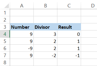
We know that 9 is divisible by 3 and gives 0 as our remainder. We get the same result when using the formula =MOD(A4, B4) in cell C4.
However, if we copy the formula in cell C5, we get the result as 1. This is because the calculation goes as 2 x 4, which gives 8 (nearest value to our dividend), which is then subtracted from our ‘number’ parameter, i.e., 9 - 8, leading to a remainder of 1.
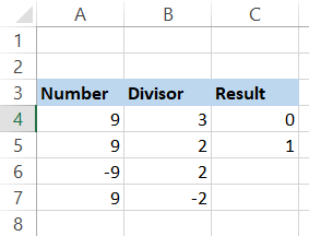
What will happen if our number is negative, like in cell A6? Will we get a negative result?
Actually, no. The result always takes the sign of the divisor. So only if the sign of the divisor is negative, as in cell B7, you can expect a negative result or a remainder from the MOD function.
Returning nth row using the MOD function
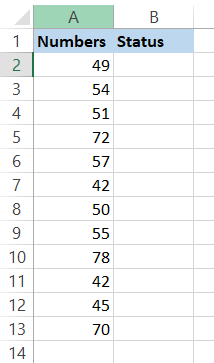
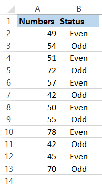
Let’s assume that you have some numbers in your Excel spreadsheet. All the cell values in the odd-numbered cells (3, 5, 7, 9…) are the junk data, while only the values in even-numbered cells (2, 4, 6, 8…) are what you require to crunch some numbers.
Here you use the combination of three functions, MOD, ROW, and IF, to help you highlight the even-numbered cells. The formula you will be using is =IF(MOD(ROW(A2), 2)=0, "Even", "Odd").
Here, our ‘number’ argument is the row number in the spreadsheet, and the divisor is 2. So whenever the MOD function encounters an even-numbered row, i.e., 2, 4, 6, 8, 10, the remainder for the function will be zero.
The IF function takes the value 0 and returns it as ‘Even’. If MOD encounters odd-numbered rows, i.e., 1, 3, 5, 7, the remainder will be one which will be displayed as ‘Odd’ in column B under the header of Status. This is what our spreadsheet looks like after implementing the above formula:
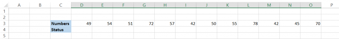
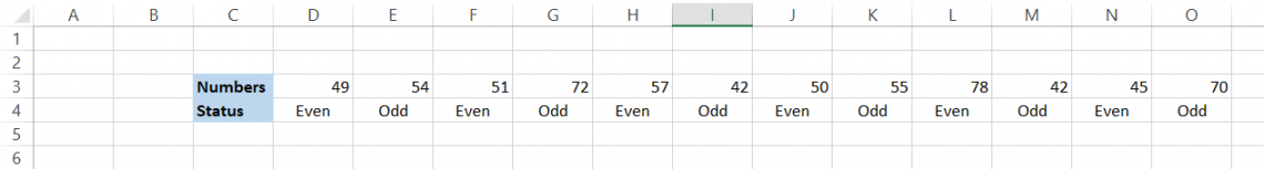
Returning nth column using the MOD function
Since you have a better understanding of how we had returned the nth row, we hope that you must have guessed what we are expecting to return the nth column. This is what our spreadsheet looks like:
The formula that we will be using is similar to the one while finding the nth row. The only major difference that we make is using the function COLUMN instead of ROW.
The formula becomes =IF(MOD(COLUMN(D3), 2)=0, "Even", "Odd") where if the MOD function encounters an even-numbered column, i.e., 2, 4, 6, 8, 10, the remainder for the function will be zero.
The IF function takes the value 0 and returns it as ‘Even’.
If your divisor would have been 3, you will get the remainders as illustrated below by using the formula =(MOD(COLUMN(D3), 3)).
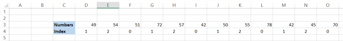
Based on the remainder that you can get, you can set up additional functions such as returning the SUM for all the numbers with the remainder as 2, or COUNTIF the numbers are greater than 50 if their remainder is 1. We shall see those examples in-depth in the following few sections.

SUM along with MOD
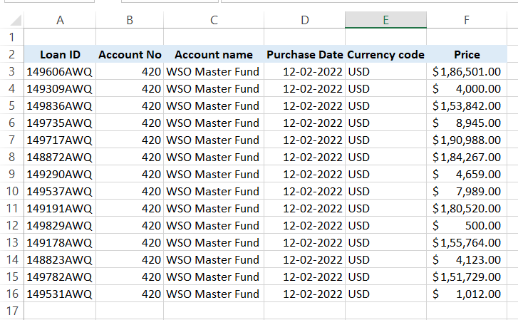
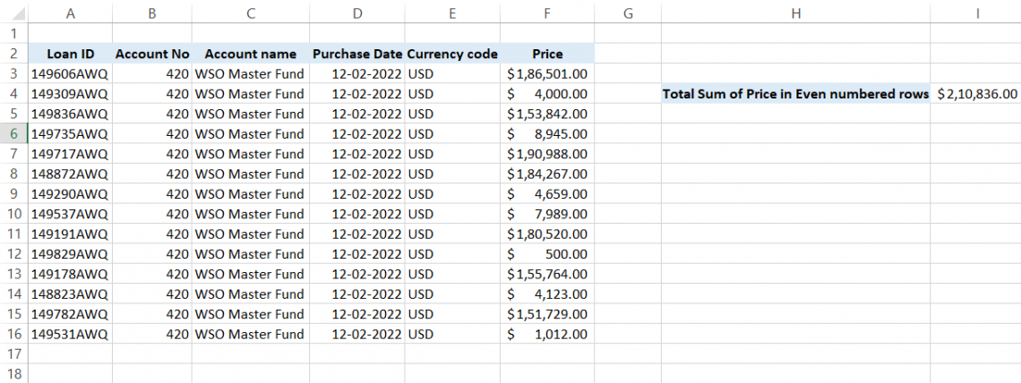
Assume that you have the following loan data for some fixed income securities and need to calculate the total price of all the securities in even-numbered rows, i.e, 2, 4, 6.
For this, you would use the formula =SUM(F3:F16*(MOD(ROW(F3:F16), 2)=0)), where the SUM range will apply only to the rows where MOD returns the remainder as zero.
This will add all the values in the cells F4, F6, F8, F10, F12, F14, F16, respectively, to give you the result of $210,836. Since this is an array formula, you must press Ctrl + Shift + Enter to get the result for the formula.
Practical Example #1
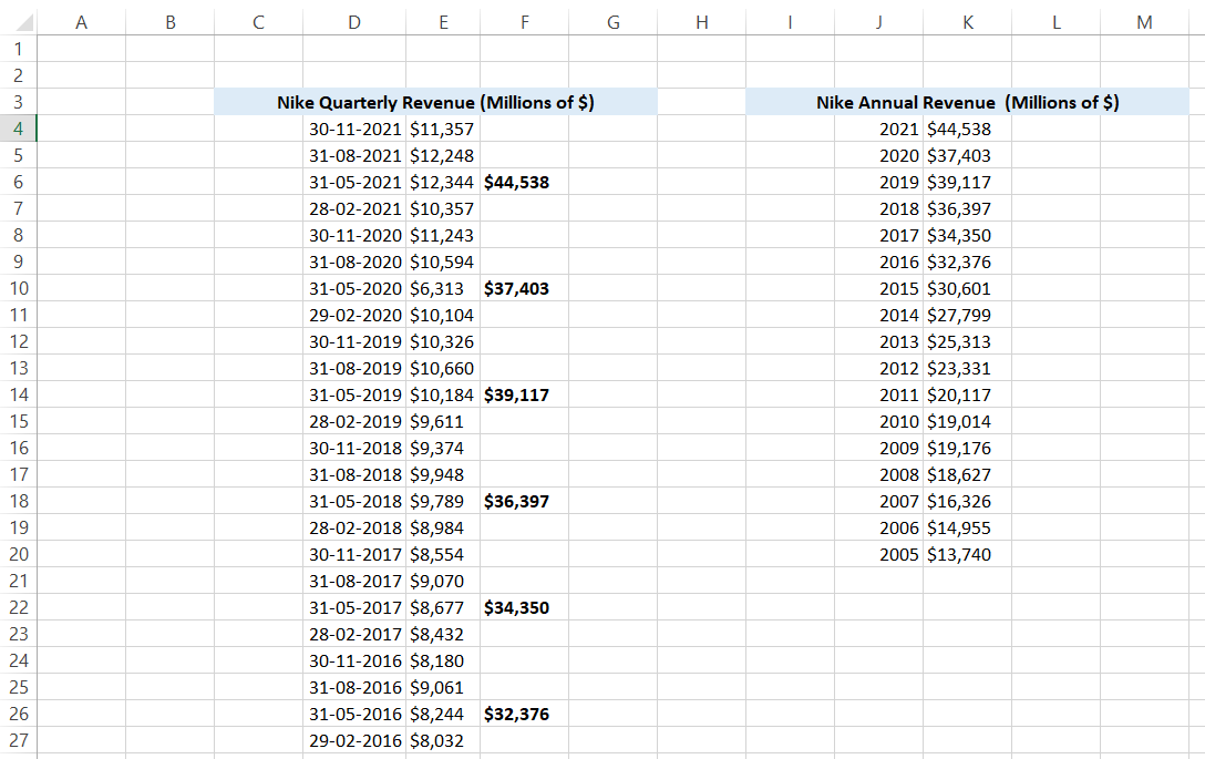
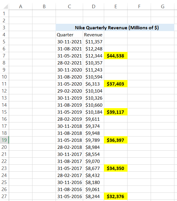
So let’s assume that we have the quarterly revenue data for Nike Inc from 2005 to 30th November 2021. Also, in another table, we have the annual revenue for Nike from 2005 to 2021.
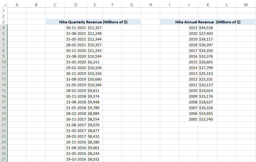
You are aware of Nike’s financial year-end date, which is 31st May every year. Now, you must link the annual revenue to the quarterly revenue table based on the fiscal year-end date.
First, we will be using the MONTH function to get the serial numbers of quarterly revenue table dates. So the formula used in the cell will be =MONTH(D4). As per our understanding, the annual reports are generally published on 31st May for Nike.
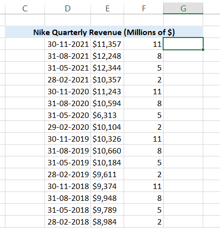
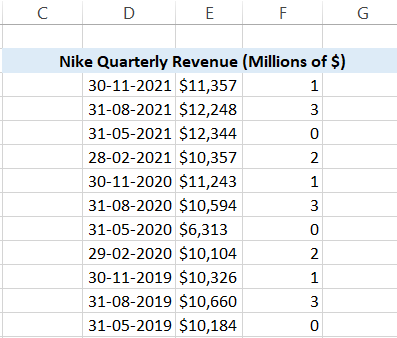
The serial number returned using the MONTH function for fiscal year-end is 5. Next, we include MOD. Since we only want the fiscal year dates to have the annual revenue value, our formula will become (MOD(MONTH(D6), 5). So now, every May month value will return the result as zero.
Next, we pull the annual revenue value from the second table using the VLOOKUP function. Our formula becomes =MOD(MONTH(D4), 5)=0, VLOOKUP(YEAR(D4), $M$4:$N$20, 2, FALSE). This means that only when the remainder is zero will the VLOOKUP fetch the value from the corresponding table and display it in column F.
We have also used the YEAR function, which gives us the serial number for the year for the referenced date. Again, this is to match our data in column M. Finally, we use the IF function to keep the cell blank if the quarter is not the same as the fiscal year-end, i.e., 31st May.
Our final formula becomes =IF(MOD(MONTH(D4), 5)=0, VLOOKUP(YEAR(D4), $M$4:$N$20, 2, FALSE), “”), as a result of which our spreadsheet looks as below:
Practical Example #2
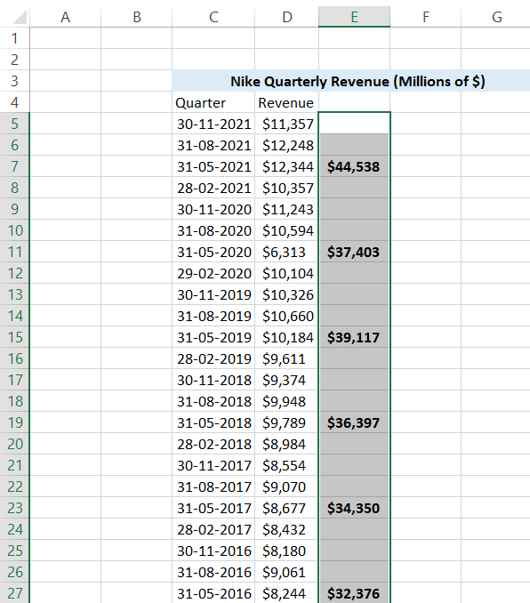
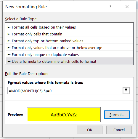
Conditional formatting and the MOD function together work great as well. For example, suppose you need to highlight the cells containing the annual revenue. First, select the range where you wish to apply the conditional formatting, i.e., E5 to E27 in our case.
Next, click on the Home tab and then select Conditional formatting. Finally, click on the New Rule option to open the dialog box. You can also use the keyboard shortcut Alt +H + L + N to open the dialog box as below:
Here, we will be selecting the Rule type as ‘Use a formula to determine which cells to format’ by clicking on it. Once it opens, we will add our formula as =MOD(MONTH(C5),5)=0 and select the background color for the cells as Yellow, which fulfills the formula criteria. Press Ok.
This is how our spreadsheet will look like after the Rule that we have set up using the conditional formatting works:
Sometimes, you might not get the result for the conditional formatting rule due to one of the common referencing errors. You need to press the keyboard shortcut Alt + H + L +R or click on the Conditional Formatting and then on Manage Rules.
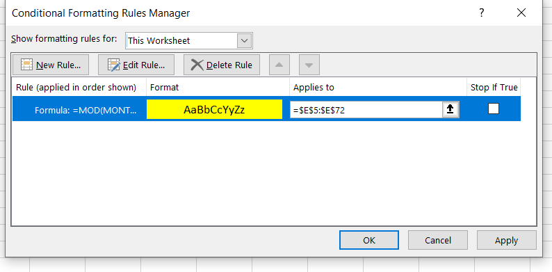
You will see the rules you have created in the This Worksheet dropdown. Now check the Applies to the box. If the cells are not properly referenced, make the changes and click on Apply. Once you do this step, you will see that the MOD formula's conditional formatting works!
A few things to remember
- You will get a #DIV/0 error when the divisor in MOD is zero.
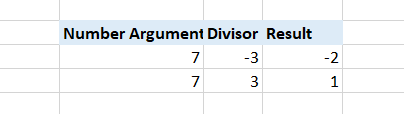
- You may get a different remainder based on the negative sign before the divisor. For example, if the ‘number’ argument is 7 and your divisor is 3, the remainder returns as 1. However, if you flip the sign for the divisor to make it -3, your remainder returns -2.

Free Resources
To continue your journey towards becoming an Excel wizard, check out these additional helpful WSO resources.

or Want to Sign up with your social account?